A Measured Response to Bentham's Bulldog

Bentham’s Bulldog writes with the confidence of a mathematician and the rigor of a theologian—which is to say, he gets it exactly backwards. I exaggerate for effect, of course, he has a great newsletter, which you should read. I thoroughly enjoy his style, themes, and the touch of philosophy. But he loves to invoke Bayesian probabilistic reasoning to argue for the existence of God, most powerfully via the fine-tuning argument, and I just hate this.

Let me briefly introduce the argument, and we’ll get to the specifics later. The argument holds that the specific values of physical constants, like the cosmological constant or the strength of gravity, fall in a very narrow range necessary for life to exist (they are “fine-tuned”). This is quite surprising, and strong evidence for a creator deity fine-tuner.

In The Fine-Tuning Argument Simply Works, he claims to have examined all objections to fine-tuning and found them wanting. He concludes that fine-tuning provides “ridiculously surprising and crazy strong evidence for God.” He claims that “there are lots of objections to [fine-tuning] but none of them work.” His arguments are wrong, I will demonstrate why, and we will learn a little measure theory.

Actually, since the whole theme of this article is precision, that doing “math via English” is perilous, let me be more clear.

Bentham’s Bulldog argues that we should believe God exists, based on the specific values of natural constants (e.g. mass of the Higgs boson, speed of light, cosmological constant). He holds that the values of these constants are fine-tuned to support life in a surprising fashion, and that the best explanation for this is that a designer (i.e. God) fine-tuned them to do so. He deploys Bayesian probability (also called “subjective” probability, inverse probability, etc.) in support of this argument. He is not the only one, here is the Stanford Encyclopedia of Philosophy’s entry detailing proponents and formulations of this argument, which are more or less identical.

Bentham’s Bulldog makes invalid arguments. The fine-tuning argument as stated in terms of Bayesian inference should neither increase nor decrease your belief in a creator, because it is mathematically meaningless. Not difficult, not imprecise—it is meaningless. It can only be rescued by abandoning the rigor of Bayesian inference (which is called something nebulous like “epistemic probability” in the Encyclopedia).

I make no claims about whether God exists. If you want theology, you should talk to a priest. Instead, let’s talk about a pervasive problem in (popular and professional) philosophy: attempting to do mathematics through English prose.

Fair Warning: This post has a lot of math and a lot of footnotes, most of which are snippy comments, but some of which are interesting.

Let's start by doing Bayesian inference correctly, on a well-defined problem. I will also introduce some measure theoretic language to aid us.

Problem Statement: You're presented with an urn containing red and blue balls. I tell you it's either type “even” (50% red, 50% blue) or type “uneven” (10% red, 90% blue). You draw one red ball. Which type of urn is it more likely to be, even or uneven?

This has a clean answer and a good method of inference. We apply Bayes’ theorem with equal priors.

Bayes' theorem is the following statement:

In English, the probability of A occurring, conditional on B being true P(A|B), is equal to the probability of B occurring, conditional on A being true P(B|A), times the ratio of the independent probabilities P(A)/P(B).

Here's the correct Bayesian calculation:

• P(even) = P(uneven) = 1/2 (no prior information favoring either)

• P(red|even) = 1/2 (by definition)

• P(red|uneven) = 1/10 (by definition)

• P(red) = P(red|even) × P(even) + P(red|uneven) × P(uneven) = 3/10

We now calculate the Bayes Factor K for these hypotheses. The Bayes factor is a ratio of the likelihoods of observing the data under two competing statistical models, and represents our “update” to our beliefs about the problem. It has the following definition (applied to our problem).

For our scenario, we have K = (0.5 / 0.1) = 5.

Our prior odds, before observing the data, are:

And our posterior odds, after observing the data, are updated by the Bayes factor:

This Bayes factor of 5 means observing a red ball increases the odds of “even” versus “uneven” by a factor of 5. With equal prior odds (1:1), we now have 5:1 posterior odds, giving us P(even|red) = 5/6 and P(uneven|red) = 1/6.

Now let’s do it again, on a slightly different version of the problem.

Problem Statement: You're presented with an urn. I tell you nothing about this urn. You reach in, and draw one red ball. What is the probability that it contains 50% red balls?

If you feel uncomfortable, good. You should. This isn't a hard problem or an imprecise problem. It's not a problem at all. It's a grammatically correct but meaningless arrangement of mathematical symbols, it is ill-posed. But isn’t it surprising that there’s an urn there with a red ball? Does that point to a deeper explanation? Perhaps so! But then again, perhaps not, and you definitely cannot assign probabilities to it without knowing what mixtures are possible or their distribution.

At this point, you may already see the shape of my objection, if so, feel free to stop here, my objection is indeed that fine-tuning is “Problem 2” dressed as “Problem 1.” For the rest of you, you were promised measure theory (and it’s odd that, having been promised measure theory in a blog post, you are still reading). Let’s go.

Note: Feel free to skip this somewhat technical section on measure theory, or just skim it. Frankly, I wrote this section as much to reify my own shaky understanding of it as to explain it to you, dear readers. We resume the polemic in section 3.

A meaningful statement about the probability of some event requires three things. A sample space Ω, a σ-algebra Σ, and a probability measure P. Together, (Ω, Σ) form our probability space and the measure P allows us to make likelihood calculations on that space.

The sample space is an intuitive concept—the set of possible outcomes. The σ-algebra Σ is the set of collections of outcomes to which we can reasonably talk about a probability. For example, the σ-algebra Σ necessarily includes the entire sample space Ω, because P(Ω) = 1, as well as the empty set ∅, because P(nothing happens) = 0. It also includes any subset of Ω we’d like to assign a probability.

We’ll set aside measure for the moment, and use a six-sided die as a concrete example to better understand these concepts.

The sample space is fairly obvious. We require a set of “events” that can occur, to which we want to assign probabilities. Crucially, we must be able to define this set. For a fair d6, it’s pretty simple, it can roll any of Ω = {1, 2, 3, 4, 5, 6}.

The σ-algebra Σ is also reasonably straightforward. For our d6, and indeed for any finite sample space, the power set (the set of all sets) usually suffices. We can, for example, reasonably assign probability to the set {2, 4, 6}, the probability of an even roll on a d6.

For more complex, or infinite sets, a standard σ-algebra on a sample space is the Borel set B, which is constructed from subsets (specifically simple open or closed intervals) of the sample space Ω by iterating (countably many times) a few well-behaved operations: union, intersection, and complement.

Basic set operations, from https://www.onlinemathlearning.com/union-set.html

Looking ahead, when we start assigning probability densities to sets, we will want “nice” sets where we don’t run into any contradictions—Borel sets are precisely these “nice” sets.

Finally, of course, we require a measure.

Probability requires measure theory to be well-defined. I first want to emphasize that “measuring,” that is, assigning a number to the intuitive notion of the “size” of some collection of objects, is not trivial, in face most sets are impossible to measure. Not difficult to measure, impossible to measure. This “problem of measure” illustrates why we ought to care about some level of rigor in probability.

Now generally speaking, the basic strategy of measure theory is to start with an object that we know we can measure, and build progressively more complex theory on this backbone. Usually, we take a collection of open intervals which we can measure (An interval [a,b] on the real line has length b-a), minimally cover our target set with this collection, and then add up those intervals. That’s the Lebesgue measure. But that doesn’t always work, in fact, it fails on most sets, and works only on so-called “measurable sets.”

Personally, I always feel that a concept of what something is feels most real when I see an example of how it can fail. So to clarify the idea of a measurable set, let’s look at the canonical example of an unmeasurable set, the Vitali set.

The Vitali set is built like this:

1. Take the rational numbers (Q) and shift them by a real number r. This creates a coset of numbers V_r = Q+r.

2. Do this for every real number r to get a collection of cosets, some of which may be identical (V_r1 = V_r2).

3. Now from each unique coset V_r you pick one number v, forming a set V.

The collection of those numbers V is the Vitali set.

Consider: if you shift V by any rational number V + q, you get a completely non-overlapping copy. Yet all these shifted copies, taken together, perfectly tile the interval [0,1]. Ok, well why isn’t it measurable?

Let’s try to assign the Vitali set a measure m. Since shifting it left and right shouldn't change its size (translation invariance), every shifted copy also has measure m. But then:

• If m = 0, then [0,1] is covered by countably many measure-zero sets, so [0,1] has measure 0. Contradiction: we know [0,1] has measure 1.

• If m > 0, then countably many copies each of measure m sum to infinity. But they all fit inside [0,1], which has measure 1. Impossible.

Neither the m = 0, nor m > 0 options work for the measure of the Vitali set, so we declare it non-measurable. This type of set is actually not rare at all. There are, in fact, infinitely many classes of unmeasurable sets, and indeed there are more unmeasurable sets than measurable sets.

Remarkably, despite the fact that almost all sets are unmeasurable, the sets we tend to encounter are measurable:

• All open and closed sets

• All countable sets

• Countable unions and intersections of measurable sets

• Complements of measurable sets

You now understand why “measuring” probability isn't trivial. Indeed, the measure must, you know, exist in order to make any meaningful statements about its size or the probability of God.

The probability measure P, rigorously speaking, satisfies all the normal measure properties (non-negative, etc.), but is also normalized, meaning that P applied to our whole sample space Ω is 1. When Bentham's Bulldog assigns probabilities to universe configurations, he's implicitly claiming a measure exists on an undefined space. Now recall the existence, indeed the preponderance, of non-measurable sets.

At the very least, right now you should be doubting whether your intuition, built from interacting with physical objects in 3D space, is especially reliable in abstract set theory (probability, unfortunately, is abstract set theory).

It’s odd, don’t you think, that if you pick a random subset of the real line, it is guaranteed to be unmeasurable with probability 1? Yet all the sets we use for, well, anything, are always measurable? Is P(God|measurable sets) therefore high?

Well, no. This is simply the natural consequence of the axiom of choice. There is no need to invoke an explanation beyond the axiom—it’s actually a single principle with very unintuitive consequences.

I also ought to introduce the concepts of probability density and cumulative density functions. They’re quite intuitive, so I’ll only bother for continuous random variables:

1. A probability density function (pdf) is a function f(x) where the probability of a continuous random variable X having the value x is proportional to f(x), and f(x) is normalized.

2. The cumulative density function is the probability that a continuous random variable X takes a value less than or equal to x, written as P(X ≤ x). It’s the integral of f(x).

There’s one more thing I want to note before ending the deep theory—you see that term up there, P(God|measurable sets)? This is the first time in this article where that P has a well-defined meaning. That P is the probability measure, finitely additive, normalized, etc, defined over a measurable sigma algebra on some sample space.

A central idea of the fine-tuning argument is that the physical constants that describe our world have a low probability of being chosen randomly—they are fine-tuned. Indeed, Bentham’s Bulldog says

Because there are at least 10^120 values of the cosmological constant alone, and nothing special, conditional on naturalism, about the finely-tuned one that it happens to be, the odds of fine-tuning by chance of just the cosmological constant are 1/10^120.

Not so fast, says the measure theorist, the probability of selecting any particular number from a continuous set is zero, only intervals are meaningful!

Now a clever philosopher who’s a bit knowledgeable about physics might counter “But wait! The Planck scale provides a natural discretization, so we’re not choosing from a continuous set, but picking a value from a set of discrete values!”

Oh no, responds the measure theorist. A discrete set of evenly spaced real values is in one-to-one correspondence with the integers, and there is no uniform probability distribution over the integers. You literally cannot select a random value. You must choose a finite set of them first, and your choice is arbitrary.

And so on.

Allow me to show you a very cool set, a very simple fractal actually. It’s cool, it helps show why you can’t trust your intuition about measurable sets, and it’s cool.

1. Begin with the interval [0,1] on the real line

2. Remove the middle third, leaving [0, 1/3] ∪ [2/3, 1].

3. From each remaining piece, remove its middle third.

4. Repeat forever.

A visual representation of the Cantor set, from https://graphicmaths.com/fractals/fractals/cantor-set/

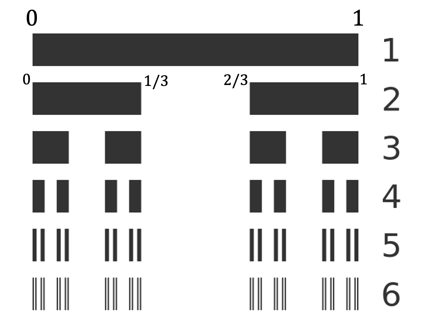
What's left—the Cantor set—has measure zero (we removed intervals totaling length 1/3 + 2/9 + 4/27 + … = 1). Yet it contains uncountably many points, as many as the original interval. It is dust that takes up no space but is everywhere dense in itself. We can even define valid probability distributions concentrated entirely on this measure-zero dust! I don’t know about you, but this is not intuitive to me at all.

A plot of the Cantor set’s cumulative distribution function is called the Devil’s Staircase. Its derivative is zero almost everywhere (except on a set of measure zero), but it still climbs!

Okay, we finally get to the meat of the essay. What is the fine-tuning argument, as stated by Bentham’s Bulldog?

I’ll actually let him state a lot of it, because he does a good job laying out the premises.

Premise 1: “The parameters of the universe are finely tuned in the sense that they fall in a very narrow range needed for life.”

Note that he distinguishes three types of fine tuning. Four, actually, if you include his mention of Robin Collins’ work on fine-tuning for discoverability.

1. Nomological Fine-Tuning (the laws themselves): Most conceivable physical laws would produce either trivial patterns or random chaos. Laws capable of generating complex, stable structures represent a vanishingly small subset of logical possibilities.

2. Constant Fine-Tuning: Physical constants fall in narrow life-permitting ranges:

   • Cosmological constant: fine-tuned to 1 part in 10^120

   • Strong nuclear force, electromagnetic force, quark masses, etc. all require precise values for complex structures.

3. Initial Condition Fine-Tuning: The universe's low-entropy starting state represents 1 part in 10^10^123 of possible configurations.

4. Fine-tuning for discoverability (Robin Collins): The values of physical constants are optimized for scientific discovery by humans.

Premise 2: This fine-tuning is highly improbable given naturalism/atheism.

“If there is a God, then the universe being finely tuned makes sense. God would want to create a universe capable of sustaining life.”

Premise 3: This fine-tuning is expected given theism (God would create life-friendly conditions).

“The odds of fine-tuning conditional on naturalism are extremely low.” By naturalism, let’s just take this to mean not-God.

Note that this is a probabilistic argument, and that Bentham’s Bulldog explicitly endorses Bayesian epistemology, so I don’t think I’m being uncharitable as reading this as Bayes’ theorem here.

If I may, let me just restate the argument, as I understand it, with math. His argument is precisely a statement that the Bayes Factor for fine-tuning is large under theism and not naturalism.

We expand via Bayes’ theorem to get our posterior odds…

So indeed, were this calculation well defined, we should update our beliefs in favor of theism!

But wait! Stop right there! Can we do this at all? Primed with that interminable section on measure theory above, we answer: no, we cannot. Remember that probability has a well-defined meaning; that P symbol is a measure, not the English phrase “the probability of”!

Now, the priors, P(God) and P(¬God), are perfectly well-defined—they're your initial degrees of belief, and you can assign what you like. The problem is the “likelihoods,” particularly P(finetuning∣¬God). To define this likelihood—the probability of fine-tuning given naturalism—you must specify a probability space. That means:

• A sample space Ω (all possible values the constants could take)

  • Real numbers? Positive only? Complex? We have no idea, and exactly one example of a universe to guess from.

• A σ-algebra Σ (which subsets we can measure)

  • Same problem.

• A probability measure P on Σ

  • If the constant can be any real number, there's no uniform distribution over ℝ. If we restrict to [0, M] for some M, why that M? Why uniform rather than log-uniform or Gaussian?

We have none of these. The Bayes Factor derived from it is meaningless.

Now there’s a possible objection to this. If P(fine-tuning∣¬God) = 0 and P(fine-tuning∣God) > 0, then the Bayes Factor K would be infinite.

But by construction, you get P(fine-tuning∣¬God) = 0 due to selecting a value from a set of zero measure (in this case, selecting a value from a continuous range). By the premise of this whole argument, then God too must select, whether randomly or not, from a set of zero measure. The probability of God selecting any particular value, P(fine-tuning∣God), is therefore also zero and the Bayes Factor is undefined.

This discussion of math is entirely apart from the problem of whether P(fine tuning|God) has any theological meaning at all, as it requires us to what God would do given some motivation. Bentham’s Bulldog argues that fine-tuning implies an omnipotent selector, but shouldn’t an all-powerful, all-math-loving being want his universe to emerge naturally from a deep symmetry?

From that perspective, our apparently 'fine-tuned' and perhaps 'contrived-looking' universe might even be considered less likely under such a conception of God. To assert a high P(fine-tuning|God) is not a neutral step; it embeds significant, debatable, and ultimately non-quantifiable theological assumptions about divine motivations and aesthetic preferences.

Should we therefore assign P(fine tuning|God) = 0 because our universe appears fine-tuned and ugly? I have no idea, neither do you, and stop assigning probabilities to theologically opaque propositions as if they were well-defined events.

Let's briefly talk about what I think is a very similar mistake in his other writing. I won’t go into too much detail, because it’s a bit outside my bailiwick, but I think it’s illustrative of the same mistake. Bentham’s Bulldog is fond of the self-indication assumption (SIA), which is a somewhat technical argument that you should condition your likelihoods on the fact that you exist.

Specifically, he argues for the “Unrestricted” version of SIA (USIA), which cares about absolute numbers of people, not just the share of possible people who exist.

1. God, being perfectly good and omnipotent, would create the maximum possible number of people. He argues this number is “unsetly many” (too large to be a mathematical set) - at minimum Beth 2, but likely much larger.

2. Even the most generous naturalistic scenarios (infinite multiverse, infinite universe) can only produce aleph-null people - the smallest infinity.

3. Beth 2 is infinitely larger than aleph-null. There are vastly more ways for you to exist if Beth 2+ people exist than if only aleph-null exist.

Your existence is therefore infinitely more likely under theism than naturalism. Even if you assign theism very low priors, an infinite Bayes factor overwhelms any finite prior probability ratio.

He writes several thousand words of increasingly baroque thought experiments and arguments by analogy defending this position, a lot of which appear convincing, but… I mean, do I have to say it? Bentham's Bulldog sees SIA predicting absurdities under naturalism and concludes theism. I see SIA predicting absurdities under ill-defined probability distributions and conclude that having well-defined probability distributions is important to avoid concluding nonsense. It's Problem 2 dressed as Problem 1, again.

I think the similarity of these two arguments reveals the deeper flaw in his arguments generally—his tendency to treat probability statements as meaningful just because they're grammatically correct.

But let it not be said that Bentham’s Bulldog is a casual writer, he thinks through the possible objections to his argument quite thoroughly! I argue he does so incorrectly, but that’s rather the topic of debate, isn’t it? I’ll go through my major gripes with his objections.

He first attempts to head off objections like mine by distinguishing between “objective chances and subjective chances.” He essentially identifies objective probability as the frequentist interpretation of long-run frequency in many trials, which he rightly dismisses as not useful with a single universe to extrapolate from.

The “subjective chance” he identifies is pure Bayesian.

To determine subjective chances, you should imagine a rational agent assigning probabilities to the possible outcomes before they know the actual outcomes. In the case of fine-tuning, for instance, a person who didn’t yet know what values the laws fell into would think there was a super small chance it would fall in the finely-tuned range because it could fall in any range.

Unfortunately, Bayesian probability theory requires well-defined probability spaces and measures just as much as frequentism. This does not help him. Indeed his analogies reveal the problem with his framing of fine tuning, and why I hate arguments by analogy in general.

[I]magine that we discover that several billions years ago someone built a special machine. This machine will spit out a number, determined by some undiscovered laws of physics that can’t be different. The number could be any number from 1 to 100 billion.

Imagine that we know that the person who made the machine just loves the number 6,853… Now imagine that the machine spits out the number 6,853.

Clearly, this should give us some evidence that he rigged the machine. Even though the machine, on the hypothesis that it’s not rigged, is wholly determined by the laws of physics, it’s unlikely that the laws of physics would determine 6,853—there’s nothing special about it. In contrast, he’d be much likelier to pick that number. Therefore, if the number is picked, it favors the hypothesis that it’s rigged.

This analogy has a well defined sample space, algebra, and measure. This is absolutely perfect Bayesian reasoning, and good job on him. This is “Problem 1” from our red balls in urns scenario. But fine-tuning is “Problem 2.”

Arguments from analogy fall into this trap continuously and I see it everywhere. Your analogy has to actually map onto the problem you’re analogizing, or it doesn’t work! A → B does not imply C → D if you show only that A is similar to C and B to D! You have to show the arrow, and that’s the hard part and the entire discipline category theory.

Bentham’s Bulldog fairly quickly dismisses the possible objection to the fine-tuning argument that there may be deeper, more fundamental laws that we don’t know about yet that predict fine-tuning. This is very closely related to the concepts in physics of naturalness (essentially just another name for fine-tuning of constants, like the Higgs mass and the cosmological constant) and the hierarchy problem (the observed vast difference in the “strengths” of the weak force and gravity).

Now of course, in his dismissal he gives an analogy about royal flushes in poker that have well defined probability distributions, which is wrong for the same reasons as above. But additionally, he more or less argues that the Deeper Laws objection just pushes the problem back a level.

There could be more fundamental laws resulting in any specific arrangement. It’s thus monstrously improbable that they’d produce a finely-tuned arrangement rather than the overwhelmingly more populous non-finely-tuned arrangements.

This is where he and I just irreconcilably disagree.

Maybe it’s just because I’ve been reading so much of his stuff writing this article, but let’s look at an analogy.

Group theory is the area of mathematics most deeply concerned with symmetry, and therefore very relevant for physics. The Classification of Finite Simple Groups is a triumph of modern mathematics, and it says that we can uniquely classify every finite, simple group (group building blocks that are not decomposable into simpler groups) into one of of four classes, the first three of which have infinitely many members.

There are the cyclic groups, the alternating groups, Lie groups, and exactly twenty-six exceptions, called the sporadic groups. Now I want you to imagine you know nothing about math, but lots about fine-tuning, and listen to this argument.

There are these four classes of groups, right?

The cyclic groups are simple to understand, they're derived from the symmetries of rotating (prime) polygons. A pentagon has 5 rotational symmetries, so the cyclic group C₅ has exactly 5 elements.

The alternating groups are the symmetry groups of even permutations of objects. If you have 5 objects, there are 5!/2 = 60 ways to rearrange them using an even number of swaps, so A₅ has exactly 60 elements.

Lie groups are concerned with continuous symmetries, like rotations in 3D space—SO(3) has dimension 3 because you need 3 numbers to specify a rotation in 3D. They each have dimensions and element counts that flow directly from the objects they describe.

Then there's the sporadic groups. There's subclasses here, actually, where some of them have good, less simple, but intuitive explanations. And then there’s the monster.

From 3blue1brown’s excellent video on the monster group.

The monster group has exactly 808,​017,​424,​794,​512,​875,​886,​459,​904,​961,​710,​757,​005,​754,​368,​000,​000,​000 elements, and the smallest faithful (complex) representation lives in a 196,883 dimensional vector space.

In a very real sense, this is more “fine-tuned” and less natural than any physical constant—this is one of the fundamental, irreducible building blocks of group theory, it’s exact to the last digit, and it just happens to be of order 8 x 10^53. Most of the other groups we usually care about have orders of, like, six.

Is this natural? Well in one sense, yes, absolutely. This is a direct consequence of the definition of a finite simple group. If you have a collection of objects with a group multiplication operation, and you require them to be associative, have an identity element, and have an inverse, the monster group is fully implied by this definition. While true, however, this explanation isn’t all that satisfying.

In another sense, of course, this is monstrously unnatural, and I want a better explanation, one that makes the connection seem inevitable. Why do these unbelievably simple axioms necessarily imply that there are exactly twenty six groups out of an infinite set that don’t fit a good pattern, and one of them has exactly ~8 x 10^53 elements?

Well, I could make a very convincing fine-tuning argument out of this. After all, what’s the probability that such a thing would occur by chance? Small, surely, unless God decreed it by fiat? One might even be tempted to calculate a Bayes factor…

Fortunately, mathematicians don’t do this. The fine-tuning of your theory is a defect, not a result, and in 1978 a really, really bizarre connection was found between the monster group and modular forms from the (seemingly) totally unrelated field of complex analysis, called “monstrous moonshine,” and it won a Fields medal.

What about the objection that this merely pushes the tuning back to the level of choosing axioms? But the claim that these undiscovered fundamental axioms would have to be “chosen” from a “vast space” of mostly non-life-permitting axioms is merely to re-assert the original probabilistic fallacy at a meta-level. The lesson from mathematical structures like the Monster group is precisely that profound specificity and apparent fine-tuning in the outcome can be an intrinsic, necessary, and non-contingent property of a system defined by (perhaps simple) fundamental rules.

So no, I do not accept his criticism that it is “monstrously improbable” when simple laws produce unbelievably unintuitive results. Mathematicians have the advantage of being able to define their axioms, and so we could see, a priori, that the monster was in fact natural somehow—it’s implicit in the group axioms. But physicists must work from the other direction, slowly digging our way down to the axioms of the universe. An appeal to theology is antithetical to the entire intellectual project of physics. It is not victory, but surrender.

Our physical models are fine-tuned. This is inarguably true, because they are fine-tuned by us, physicists, to match the empirical results we get from interacting with the world. The work of the physicist is to improve the map, and not to confuse it for the territory.

Let me be crystal clear.

• I am not arguing that a creator does not exist.

• I am not arguing that the universe itself doesn’t appear fine-tuned in a nomological, initial conditions, or universal constants sense.

• I am not arguing that this isn’t deeply puzzling and cries out for an explanation.

But none of this is Bayesian evidence for a creator. Nor is it evidence against one, because it is not Bayesian evidence at all. Instead, Bentham’s Bulldog appeals to probability theory's language and authority without accepting its constraints. He does math with English instead of math, and his arguments are wrong.

The honest position is this: we don't know how to assign probabilities to fundamental physics. We have exactly one universe, incomplete understanding of its laws, and no way to define the space of “possible physics.” The fine-tuning observation may be TRUE—the constants may indeed fall in a narrow life-permitting range for no good reason and there may indeed be a God who made it that way! But the argument that fine-tuning provides calculable evidence for God is not VALID—it relies on undefined probability distributions over undefined spaces.

With that, I rest my case. I hope you enjoyed it.