A Researcher's Field Guide to Non-Standard LLM Architectures

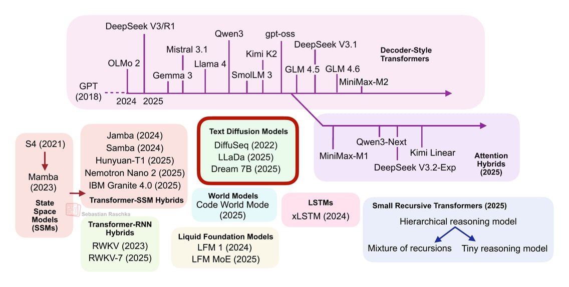
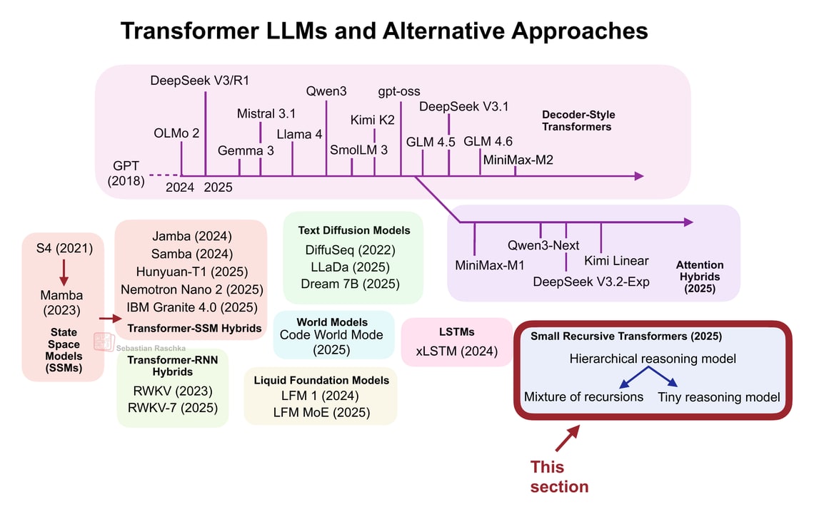
From DeepSeek R1 to MiniMax-M2, the largest and most capable open-weight LLMs today remain autoregressive decoder-style transformers, which are built on flavors of the original multi-head attention mechanism.

However, we have also seen alternatives to standard LLMs popping up in recent years, from text diffusion models to the most recent linear attention hybrid architectures. Some of them are geared towards better efficiency, and others, like code world models, aim to improve modeling performance.

After I shared my Big LLM Architecture Comparison a few months ago, which focused on the main transformer-based LLMs, I received a lot of questions with respect to what I think about alternative approaches. (I also recently gave a short talk about that at the PyTorch Conference 2025, where I also promised attendees to follow up with a write-up of these alternative approaches). So here it is!

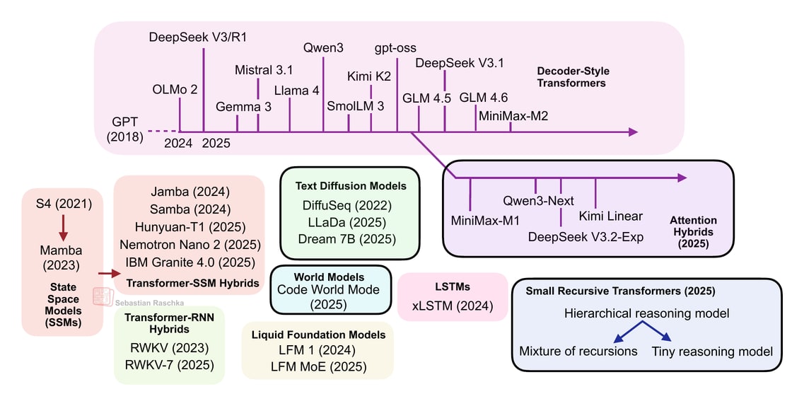
Note that ideally each of these topics shown in the figure above would deserve at least a whole article itself (and hopefully get it in the future). So, to keep this article at a reasonable length, many sections are reasonably short. However, I hope this article is still useful as an introduction to all the interesting LLM alternatives that emerged in recent years.

PS: The aforementioned PyTorch conference talk will be uploaded to the official PyTorch YouTube channel. In the meantime, if you are curious, you can find a practice recording version below.

(There is also a YouTube version here.)

Before we discuss the “more different” approaches, let’s first look at transformer-based LLMs that have adopted more efficient attention mechanisms. In particular, the focus is on those that scale linearly rather than quadratically with the number of input tokens.

There’s recently been a revival in linear attention mechanisms to improve the efficiency of LLMs.

The attention mechanism introduced in the Attention Is All You Need paper (2017), aka scaled-dot-product attention, remains the most popular attention variant in today’s LLMs. Besides traditional multi-head attention, it’s also used in the more efficient flavors like grouped-query attention, sliding window attention, and multi-head latent attention as discussed in my talk.

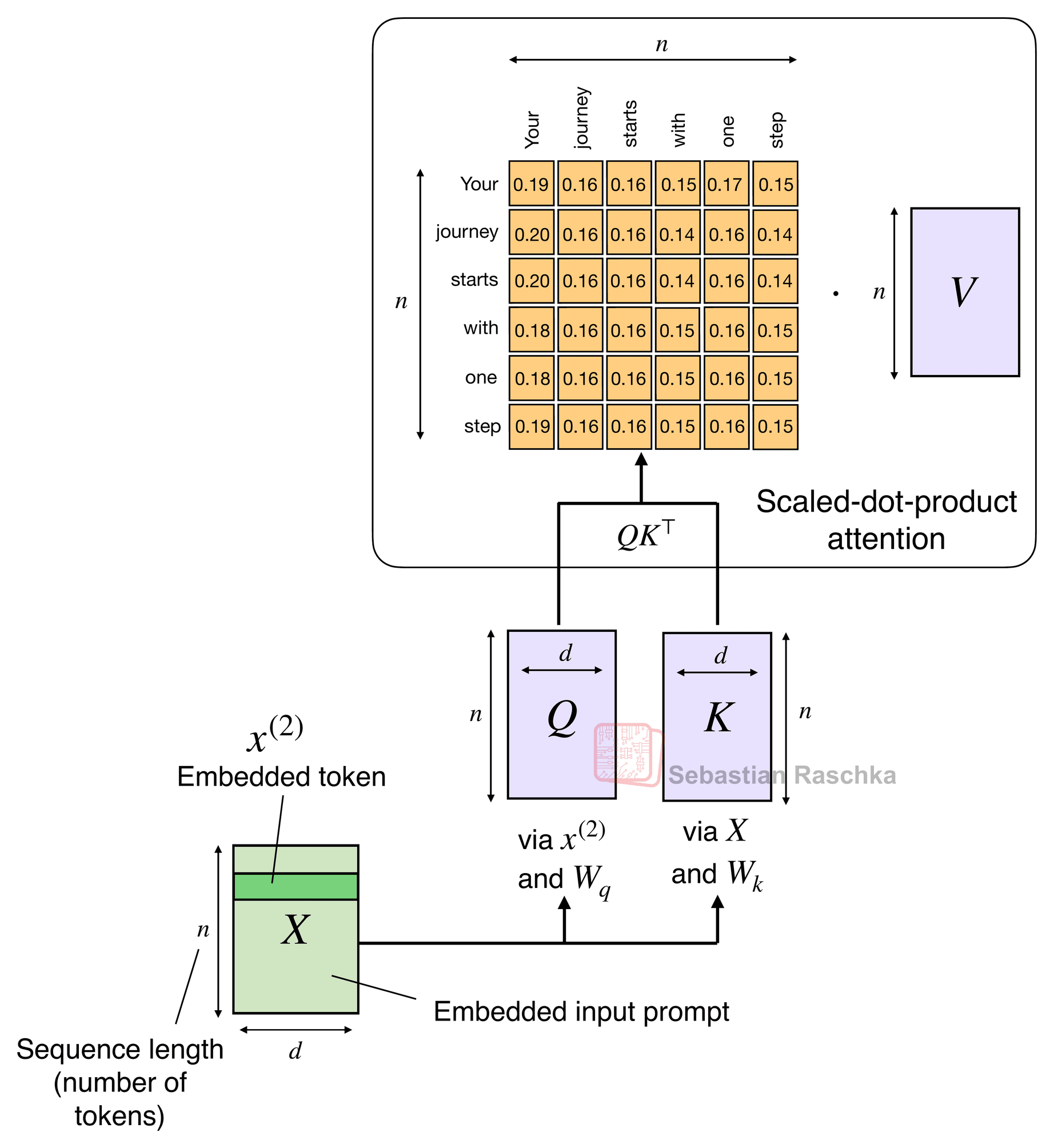
The original attention mechanism scales quadratically with the sequence length:

This is because the query (Q), key (K), and value (V) are n-by-d matrices, where d is the embedding dimension (a hyperparameter) and n is the sequence length (i.e., the number of tokens).

(You can find more details in my Understanding and Coding Self-Attention, Multi-Head Attention, Causal-Attention, and Cross-Attention in LLMs article)

Linear attention variants have been around for a long time, and I remember seeing tons of papers in the 2020s. For example, one of the earliest I recall is the 2020 Transformers are RNNs: Fast Autoregressive Transformers with Linear Attention paper, where the researchers approximated the attention mechanism:

Here, ϕ(⋅) is a kernel feature function, set to ϕ(x) = elu(x)+1.

This approximation is efficient because it avoids explicitly computing the n×n attention matrix QK^T.

I don’t want to dwell too long on these older attempts. But the bottom line was that they reduced both time and memory complexity from O(n²) to O(n) to make attention much more efficient for long sequences.

However, they never really gained traction as they degraded the model accuracy, and I have never really seen one of these variants applied in an open-weight state-of-the-art LLM.

In the second half of this year, there has been revival of linear attention variants, as well as a bit of a back-and-forth from some model developers as illustrated in the figure below.

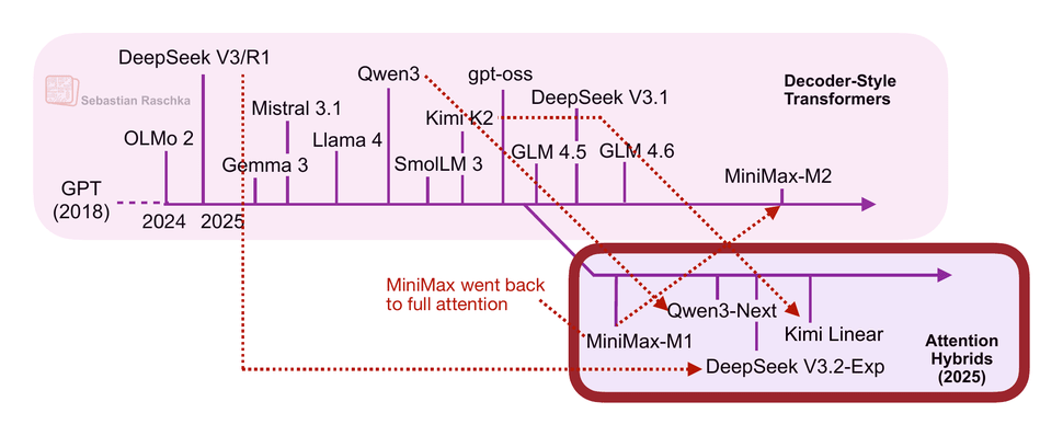
The first notable model was MiniMax-M1 with lightning attention.

MiniMax-M1 is a 456B parameter mixture-of-experts (MoE) model with 46B active parameters, which came out back in June.

Then, in August, the Qwen3 team followed up with Qwen3-Next, which I discussed in more detail above. Then, in September, the DeepSeek Team announced DeepSeek V3.2. (DeepSeek V3.2 sparse attention mechanism is not strictly linear but at least subquadratic in terms of computational costs, so I think it’s fair to put it into the same category as MiniMax-M1, Qwen3-Next, and Kimi Linear.)

All three models (MiniMax-M1, Qwen3-Next, DeepSeek V3.2) replace the traditional quadratic attention variants in most or all of their layers with efficient linear variants.

Interestingly, there was a recent plot twist, where the MiniMax team released their new 230B parameter M2 model without linear attention, going back to regular attention. The team stated that linear attention is tricky in production LLMs. It seemed to work fine with regular prompts, but it had poor accuracy in reasoning and multi-turn tasks, which are not only important for regular chat sessions but also agentic applications.

This could have been a turning point where linear attention may not be worth pursuing after all. However, it gets more interesting. In October, the Kimi team released their new Kimi Linear model with linear attention.

For this linear attention aspect, both Qwen3-Next and Kimi Linear adopt a Gated DeltaNet, which I wanted to discuss in the next few sections as one example of a hybrid attention architecture.

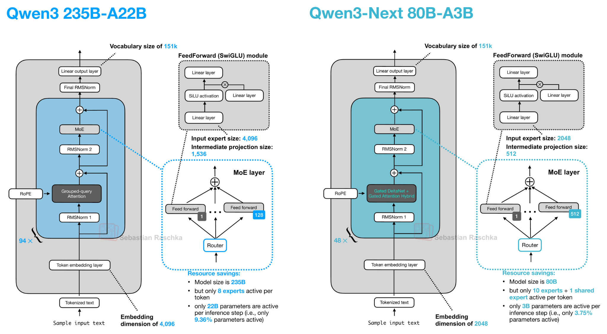
Let’s start with Qwen3-Next, which replaced the regular attention mechanism by a Gated DeltaNet + Gated Attention hybrid, which helps enable the native 262k token context length in terms of memory usage (the previous 235B-A22B model model supported 32k natively, and 131k with YaRN scaling.)

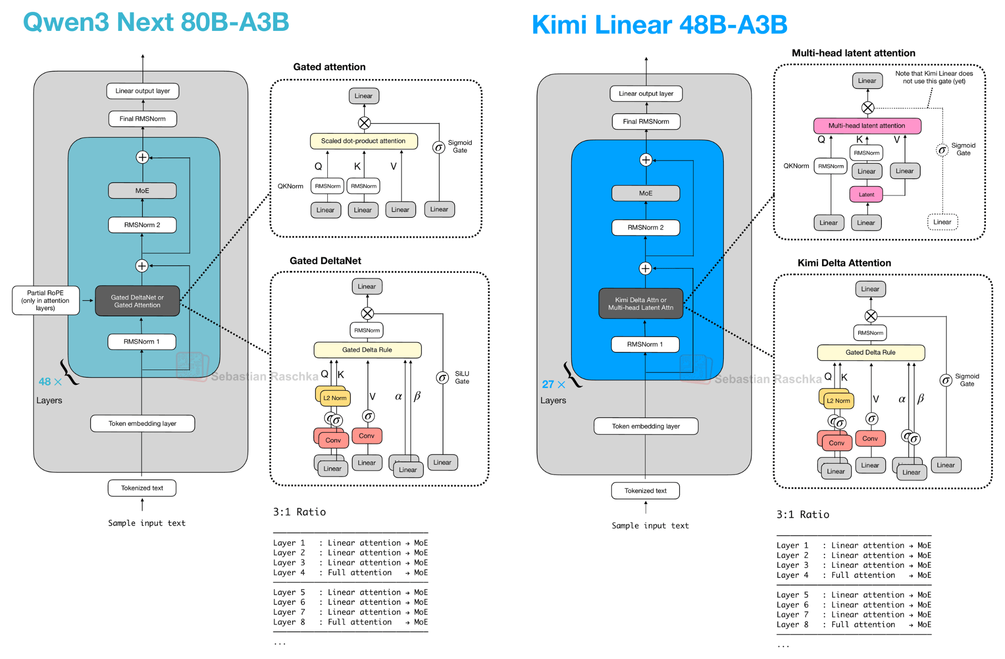
Their hybrid mechanism mixes Gated DeltaNet blocks with Gated Attention blocks within a 3:1 ratio as shown in the figure below.

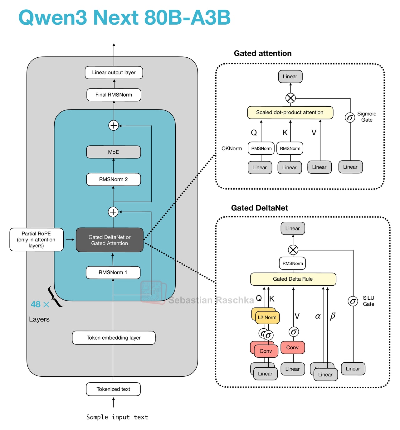
As depicted in the figure above, the attention mechanism is either implemented as gated attention or Gated DeltaNet. This simply means the 48 transformer blocks (layers) in this architecture alternate between this. Specifically, as mentioned earlier, they alternate in a 3:1 ratio. For instance, the transformer blocks are as follows:

────────────────────────────────── Layer 1 : Linear attention → MoE Layer 2 : Linear attention → MoE Layer 3 : Linear attention → MoE Layer 4 : Full attention → MoE ────────────────────────────────── Layer 5 : Linear attention → MoE Layer 6 : Linear attention → MoE Layer 7 : Linear attention → MoE Layer 8 : Full attention → MoE ────────────────────────────────── ...

Otherwise, the architecture is pretty standard and similar to Qwen3:

So, what are gated attention and Gated DeltaNet?

Before we get to the Gated DeltaNet itself, let’s briefly talk about the gate. As you can see in the upper part of the Qwen3-Next architecture in the previous figure, Qwen3-Next uses “gated attention”. This is essentially regular full attention with an additional sigmoid gate.

This gating is a simple modification that I added to an MultiHeadAttention implementation (based on code from chapter 3 of my LLMs from Scratch book) below for illustration purposes:

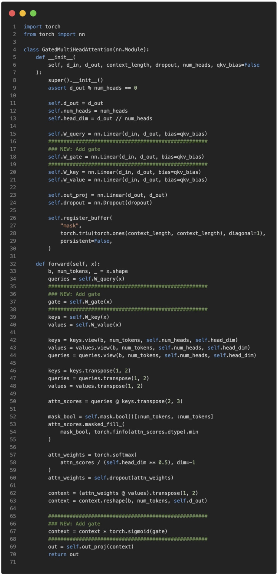
As we can see, after computing attention as usual, the model uses a separate gating signal from the same input, applies a sigmoid to keep it between 0 and 1, and multiplies it with the attention output. This allows the model to scale up or down certain features dynamically. The Qwen3-Next developers state that this helps with training stability:

[...] the attention output gating mechanism helps eliminate issues like Attention Sink and Massive Activation, ensuring numerical stability across the model.

In short, gated attention modulates the output of standard attention. In the next section, we discuss Gated DeltaNet, which replaces the attention mechanism itself with a recurrent delta-rule memory update.

Now, what is Gated DeltaNet? Gated DeltaNet (short for Gated Delta Network) is Qwen3-Next’s linear-attention layer, which is intended as an alternative to standard softmax attention. It was adopted from the Gated Delta Networks: Improving Mamba2 with Delta Rule paper as mentioned earlier.

Gated DeltaNet was originally proposed as an improved version of Mamba2, where it combines the gated decay mechanism of Mamba2 with a delta rule.

Mamba is a state-space model (an alternative to transformers), a big topic that deserves separate coverage in the future.

The delta rule part refers to computing the difference (delta, Δ) between new and predicted values to update a hidden state that is used as a memory state (more on that later).

(Side note: Readers with classic machine learning literature can think of this as similar to Hebbian learning inspired by biology: “Cells that fire together wire together.” It’s basically a precursor of the perceptron update rule and gradient descent-based learning, but without supervision.)

Gated DeltaNet has a gate similar to the gate in gated attention discussed earlier, except that it uses a SiLU instead of logistic sigmoid activation, as illustrated below. (The SiLU choice is likely to improve gradient flow and stability over the standard sigmoid.)

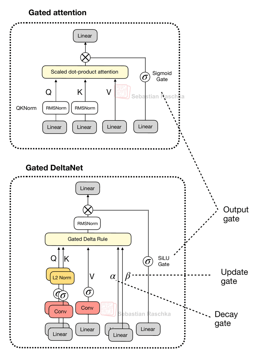
However, as shown in the figure above, next to the output gate, the “gated” in the Gated DeltaNet also refers to several additional gates:

• α (decay gate) controls how fast the memory decays or resets over time,

• β (update gate) controls how strongly new inputs modify the state.

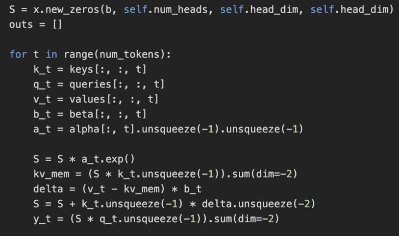
In code, a simplified version of the Gated DeltaNet depicted above (without the convolutional mixing) can be implemented as follows (the code is inspired by the official implementation by the Qwen3 team):

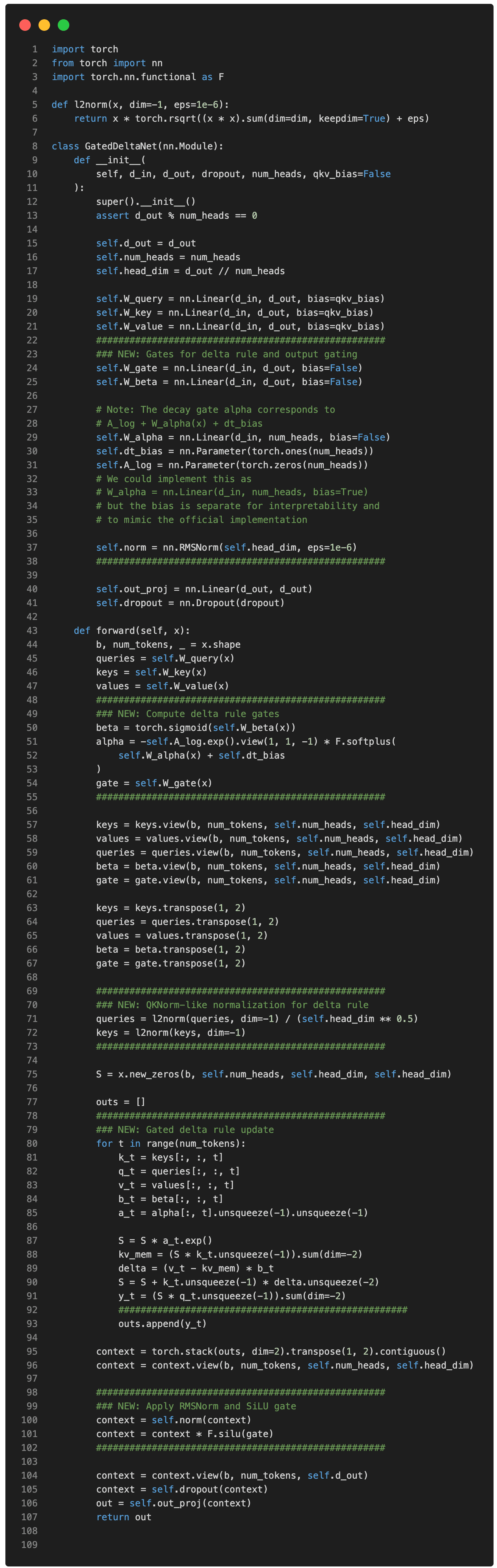
(Note that for simplicity, I omitted the convolutional mixing that Qwen3-Next and Kimi Linear use to keep the code more readable and focus on the recurrent aspects.)

So, as we can see above, there are lots of differences to standard (or gated) attention.

In gated attention, the model computes normal attention between all tokens (every token attends or looks at every other token). Then, after getting the attention output, a gate (a sigmoid) decides how much of that output to keep. The takeaway is that it’s still the regular scaled-dot product attention that scales quadratically with the context length.

As a refresher, scaled-dot product attention is computed as softmax(QKᵀ)V, where Q and K are n-by-d matrices, where n is the number of input tokens, and d is the embedding dimension. So QKᵀ results in an attention n-by-n matrix, that is multiplied by an n-by-d dimensional value matrix V.

In Gated DeltaNet, there’s no n-by-n attention matrix. Instead, the model processes tokens one by one. It keeps a running memory (a state) that gets updated as each new token comes in. This is what’s implemented as, where S is the state that gets updated recurrently for each time step t.

And the gates control how that memory changes:

• α (alpha) regulates how much of the old memory to forget (decay).

• β (beta) regulates how much the current token at time step t updates the memory.

(And the final output gate, not shown in the snippet above, is similar to gated attention; it controls how much of the output is kept.)

So, in a sense, this state update in Gated DeltaNet is similar to how recurrent neural networks (RNNs) work. The advantage is that it scales linearly (via the for-loop) instead of quadratically with context length.

The downside of this recurrent state update is that, compared to regular (or gated) attention, it sacrifices the global context modeling ability that comes from full pairwise attention.

Gated DeltaNet, can, to some extend, still capture context, but it has to go through the memory (S) bottleneck. That memory is a fixed size and thus more efficient, but it compresses past context into a single hidden state similar to RNNs.

That’s why the Qwen3-Next and Kimi Linear architectures don’t replace all attention layers with DeltaNet layers but use the 3:1 ratio mentioned earlier.

In the previous section, we discussed the advantage of the DeltaNet over full attention in terms of linear instead of quadratic compute complexity with respect to the context length.

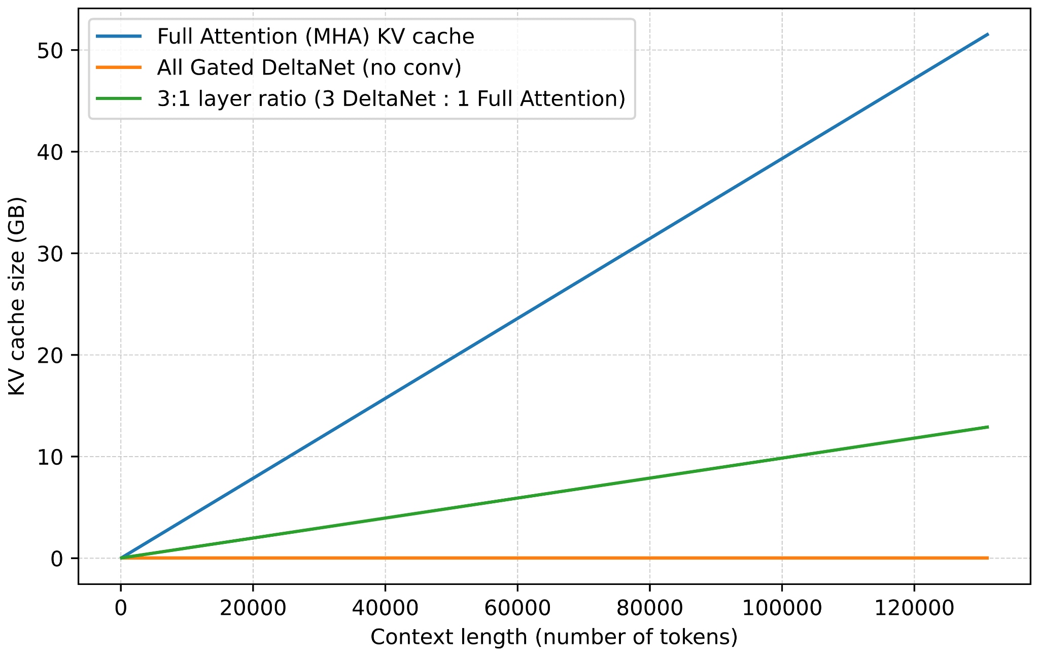
Next to the linear compute complexity, another big advantage of DeltaNet is the memory savings, as DeltaNet modules don’t grow the KV cache. (For more information about KV caching, see my Understanding and Coding the KV Cache in LLMs from Scratch article). Instead, as mentioned earlier, they keep a fixed-size recurrent state, so memory stays constant with context length.

For a regular multi-head attention (MHA) layer, we can compute the KV cache size as follows:

KV_cache_MHA ≈ batch_size × n_tokens × n_heads × d_head × 2 × bytes

(The 2 multiplier is there because we have both keys and values that we store in the cache.)

For the simplified DeltaNet version implemented above, we have:

KV_cache_DeltaNet = batch_size × n_heads × d_head × d_head × bytes

Note that the KV_cache_DeltaNet memory size doesn’t have a context length (n_tokens) dependency. Also, we have only the memory state S that we store instead of separate keys and values, hence 2 × bytes becomes just bytes. However, note that we now have a quadratic d_heads × d_head in here. This comes from the state:

S = x.new_zeros(b, self.num_heads, self.head_dim, self.head_dim)

But that’s usually nothing to worry about, as the head dimension is usually relatively small. For instance, it’s 128 in Qwen3-Next.

The full version with the convolutional mixing is a bit more complex, including the kernel size and so on, but the formulas above should illustrate the main trend and motivation behind the Gated DeltaNet.

Kimi Linear shares several structural similarities with Qwen3-Next. Both models rely on a hybrid attention strategy. Concretely, they combine lightweight linear attention with heavier full attention layers. Specifically, both use a 3:1 ratio, meaning for every three transformer blocks employing the linear Gated DeltaNet variant, there’s one block that uses full attention as shown in the figure below.

Gated DeltaNet is a linear attention variant with inspiration from recurrent neural networks, including a gating mechanism from the Gated Delta Networks: Improving Mamba2 with Delta Rule paper. In a sense, Gated DeltaNet is a DeltaNet with Mamba-style gating, and DeltaNet is a linear attention mechanism (more on that in the next section)

The MLA in Kimi Linear, depicted in the upper right box in the Figure 11 above, does not use the sigmoid gate.This omission was intentional so that the authors could compare the architecture more directly to standard MLA, however, they stated that they plan to add it in the future.

Also note that the omission of the RoPE box in the Kimi Linear part of the figure above is intentional as well. Kimi applies NoPE (No Positional Embedding) in multi-head latent attention MLA) layers (global attention). As the authors state, this lets MLA run as pure multi-query attention at inference and avoids RoPE retuning for long‑context scaling (the positional bias is supposedly handled by the Kimi Delta Attention blocks). For more information on MLA, and multi-query attention, which is a special case of grouped-query attention, please see my The Big LLM Architecture Comparison article.

Kimi Linear modifies the linear attention mechanism of Qwen3-Next by the Kimi Delta Attention (KDA) mechanism, which is essentially a refinement of Gated DeltaNet.
Whereas Qwen3-Next applies a scalar gate (one value per attention head) to control the memory decay rate, Kimi Linear replaces it with a channel-wise gating for each feature dimension. According to the authors, this gives more control over the memory, and this, in turn, improves long-context reasoning.

In addition, for the full attention layers, Kimi Linear replaces Qwen3-Next’s gated attention layers (which are essentially standard multi-head attention layers with output gating) with multi-head latent attention (MLA). This is the same MLA mechanism used by DeepSeek V3/R1 (as discussed in my The Big LLM Architecture Comparison article) but with an additional gate. (To recap, MLA compresses the key/value space to reduce the KV cache size.)

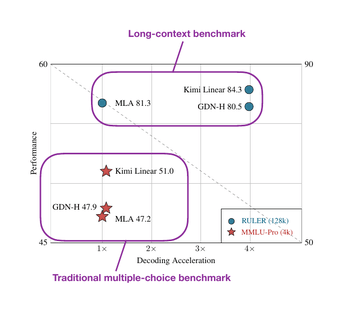
There’s no direct comparison to Qwen3-Next, but compared to the Gated DeltaNet-H1 model from the Gated DeltaNet paper (which is essentially Gated DeltaNet with sliding-window attention), Kimi Linear achieves higher modeling accuracy while maintaining the same token-generation speed.

Furthermore, according to the ablation studies in the DeepSeek-V2 paper, MLA is on par with regular full attention when the hyperparameters are carefully chosen.

And the fact that Kimi Linear compares favorably to MLA on long-context and reasoning benchmarks makes linear attention variant once again promising for larger state-of-the-art models. That being said, Kimi Linear is 48B-parameter large, but it’s 20x smaller than Kimi K2. It will be interesting to see if the Kimi team adopts this approach for their upcoming K3 model.

Linear attention is not a new concept, but the recent revival of hybrid approaches shows that researchers are again seriously looking for practical ways to make transformers more efficient. For example Kimi Linear, compared to regular full attention, has a 75% KV cache reduction and up to 6x decoding throughput.

What makes this new generation of linear attention variants different from earlier attempts is that they are now used together with standard attention rather than replacing it completely.

Looking ahead, I expect that the next wave of attention hybrids will focus on further improving long-context stability and reasoning accuracy so that they get closer to the full-attention state-of-the-art.

A more radical departure from the standard autoregressive LLM architecture is the family of text diffusion models.

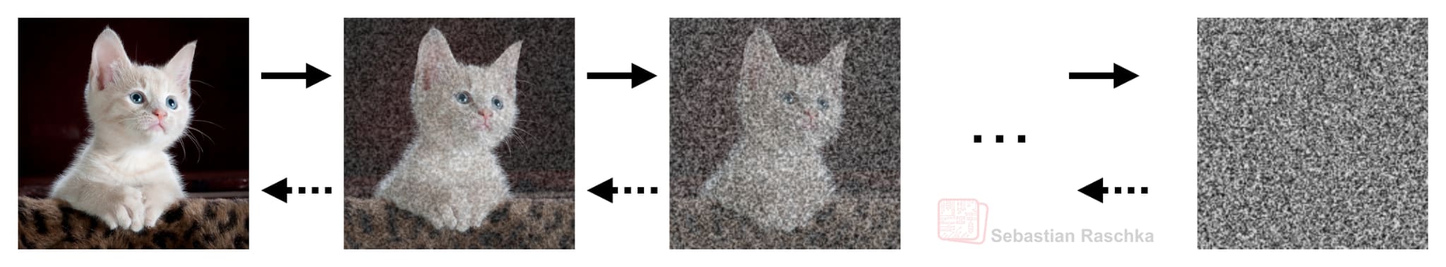
You are probably familiar with diffusion models, which are based on the Denoising Diffusion Probabilistic Models paper from 2020 for generating images (as a successor to generative adversarial networks) that was later implemented, scaled, and popularized by Stable Diffusion and others.

With the Diffusion‑LM Improves Controllable Text Generation paper in 2022, we also started to see the beginning of a trend where researchers started to adopt diffusion models for generating text. And I’ve seen a whole bunch of text diffusion papers in 2025. When I just checked my paper bookmark list, there are 39 text diffusion models on there! Given the rising popularity of these models, I thought it was finally time to talk about them.

So, what’s the advantage of diffusion models, and why are researchers looking into this as an alternative to traditional, autoregressive LLMs?

Traditional transformer-based (autoregressive) LLMs generate one token at a

time. For brevity, let’s refer to them simply as autoregressive LLMs. Now, the main selling point of text diffusion-based LLMs (let’s call them “diffusion LLMs”) is that they can generate multiple tokens in parallel rather than sequentially.

Note that diffusion LLMs still require multiple denoising steps. However,

even if a diffusion model needs, say, 64 denoising steps to produce all tokens

in parallel at each step, this is still computationally more efficient than

performing 2,000 sequential generation steps to produce a 2,000-token response.

The denoising process in a diffusion LLM, analogous to the denoising process in regular image diffusion models, is shown in the GIF below. (The key difference is that, instead of adding Gaussian noise to pixels, text diffusion corrupts sequences by masking tokens probabilistically.)

For this experiment, I ran the 8B instruct model from the Large Language Diffusion Models (LLaDA) paper that came out earlier this year.

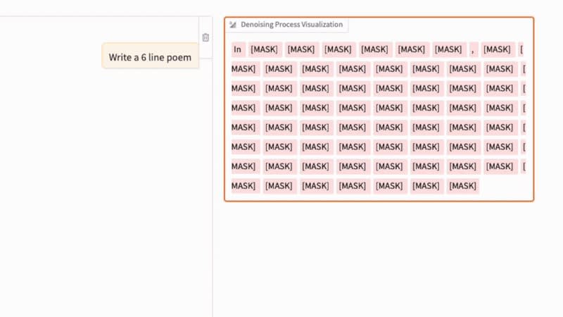
As we can see in the animation above, the text diffusion process successively replaces [MASK] tokens with text tokens to generate the answer. If you are familiar with BERT and masked language modeling, you can think of this diffusion process as an iterative application of the BERT forward pass (where BERT is used with different masking rates).

Architecture-wise, diffusion LLMs are usually decoder-style transformers but without the causal attention mask. For instance, the aforementioned LLaDA model uses the Llama 3 architecture. We call those architectures without a causal mask “bidirectional” as they have access to all sequence elements all at once. (Note that this is similar to the BERT architecture, which is called “encoder-style” for historical reasons.)

So, the main difference between autoregressive LLMs and diffusion LLMs (besides removing the causal mask) is the training objective. Diffusion LLMs like LLaDA use a generative diffusion objective instead of a next-token prediction objective.

In image models, the generative diffusion objective is intuitive because we have a continuous pixel space. For instance, adding Gaussian noise and learning to denoise are mathematically natural operations. Text, however, consists of discrete tokens, so we can’t directly add or remove “noise” in the same continuous sense.

So, instead of perturbing pixel intensities, these diffusion LLMs corrupt text by progressively masking tokens at random, where each token is replaced by a special mask token with a specified probability. The model then learns a reverse process that predicts the missing tokens at each step, which effectively “denoises” (or unmasks) the sequence back to the original text, as shown in the animation in Figure 15 earlier.

Explaining the math behind it would be better suited for a separate tutorial, but roughly, we can think about it as BERT extended into a probabilistic maximum-likelihood framework.

Earlier, I said that what makes diffusion LLMs appealing is that they generate (or denoise) tokens in parallel instead of generating them sequentially as in a regular autoregressive LLM. This has the potential for making diffusion models more efficient than autoregressive LLMs.

That said, the autoregressive nature of traditional LLMs is one of their

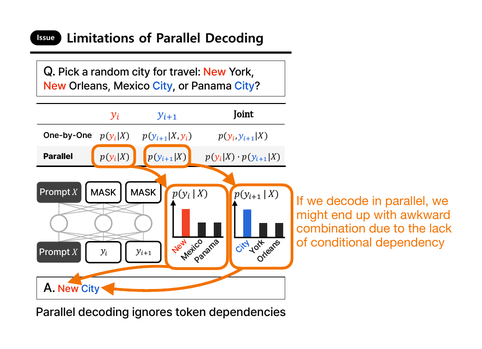
key strengths, though. And the problem with pure parallel decoding can be illustrated with an excellent example from the recent ParallelBench: Understanding the Trade-offs of Parallel Decoding in Diffusion LLMs paper.

For example, consider the following prompt:

> “Pick a random city for travel: New York, New Orleans, Mexico City, or Panama

> City?”

Suppose we ask the LLM to generate a two-token answer. It might first sample

the token “New” according to the conditional probability p(y_t = ”New” | X).

In the next iteration, it would then condition on the previously-generated token and likely choose

“York” or “Orleans,” since both conditional probabilities

p(y_t+1 = ”York” | X, y_t = ”New”) and p(y_t+1 = ”Orleans” | X, y_t = ”New”)

are relatively high (because “New” frequently co-occurs with these continuations in the training set).

But if instead both tokens were sampled in parallel, the model might independently

select the two highest-probability tokens p(y_t = “New” | X) and p(y_{t+1} = “City” | X) leading to awkward outputs like “New City.” (This is because the model lacks autoregressive conditioning and fails to capture token dependencies.)

In any case, the above is a simplification that makes it sound as if there is no conditional dependency in diffusion LLMs at all. This is not true. A diffusion LLM predicts all tokens in parallel, as said earlier, but the predictions are jointly dependent through the iterative refinement (denoising) steps.

Here, each diffusion step conditions on the entire current noisy text. And tokens influence each other through cross-attention and self-attention in every step. So, even though all positions are updated simultaneously, the updates are conditioned on each other through shared attention layers.

However, as mentioned earlier, in theory, 20-60 diffusion steps may be cheaper than the 2000 inference steps in an autoregressive LLM when generating a 2000-token answer.

It’s an interesting trend that vision models adopt components from LLMs like attention and the transformer architecture itself, whereas text-based LLMs are getting inspired by pure vision models, implementing diffusion for text.

Personally, besides trying a few demos, I haven’t used many diffusion models yet, but I consider it a trade-off. If we use a low number of diffusion steps, we generate the answer faster but may produce an answer with degraded quality. If we increase the diffusion steps to generate better answers, we may end up with a model that has similar costs to an autoregressive one.

To quote the authors of the ParallelBench: Understanding the Trade-offs of Parallel Decoding in Diffusion LLMs paper:

[...] we systematically analyse both [diffusion LLMs] and autoregressive LLMs, revealing that: (i) [diffusion LLMs] under parallel decoding can suffer dramatic quality degradation in real-world scenarios, and (ii) current parallel decoding strategies struggle to adapt their degree of parallelism based on task difficulty, thus failing to achieve meaningful speed-up without compromising quality.

Additionally, another particular downside I see is that diffusion LLMs cannot use tools as part of their chain because there is no chain. Maybe it’s possible to interleave them between diffusion steps, but I assume this is not trivial. (Please correct me if I am wrong.)

In short, it appears that diffusion LLMs are an interesting direction to explore, but for now, they may not replace autoregressive LLMs. However, I can see them as interesting alternatives to smaller, on-device LLMs, or perhaps replacing smaller, distilled autoregressive LLMs.

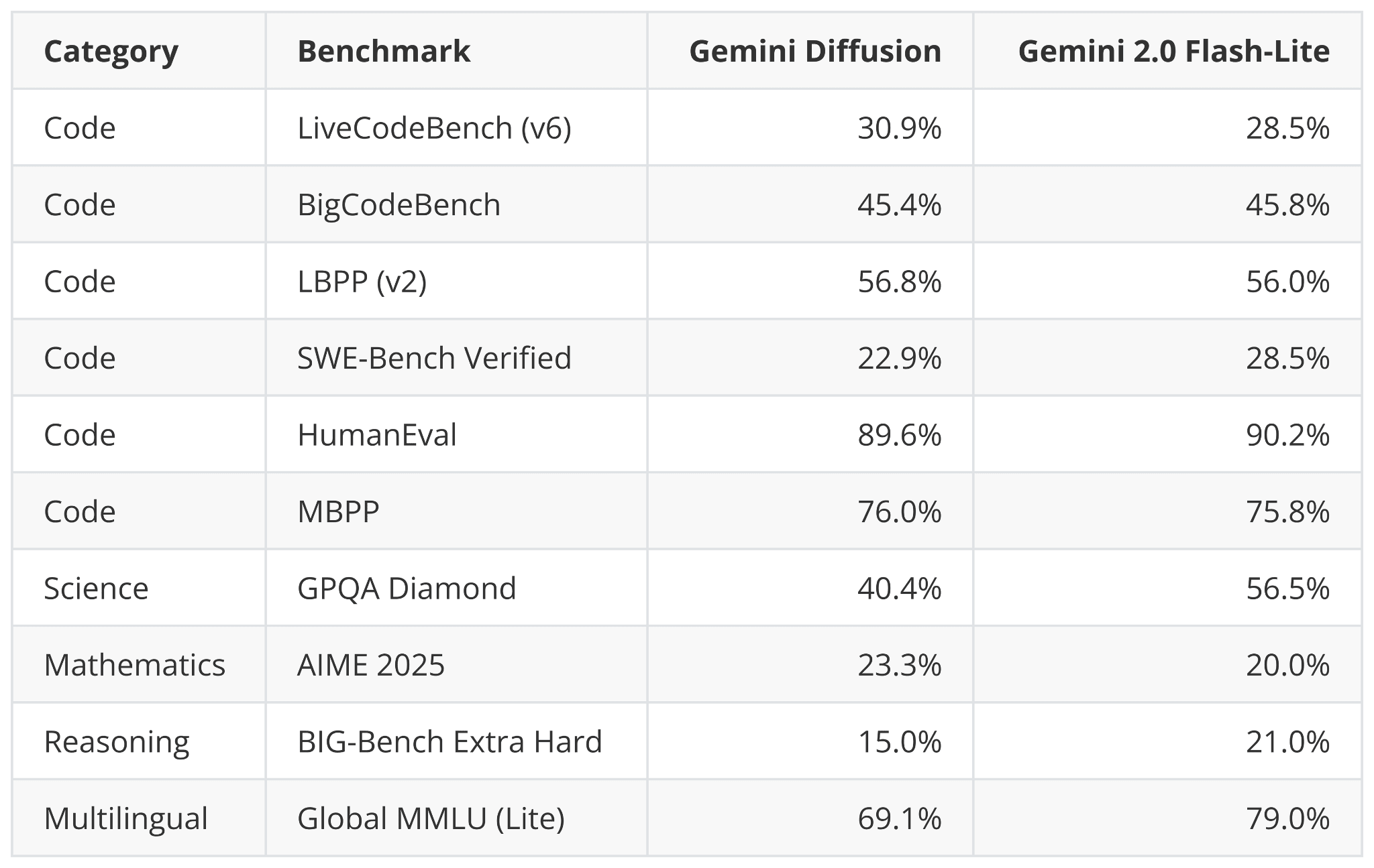
For instance, Google announced that it is working on a Gemini Diffusion model for text, where they state

Rapid response: Generates content significantly faster than even our fastest model so far.

And while being faster, it appears that the benchmark performance remains on par with their fast Gemini 2.0 Flash-Lite model. It will be interesting to see what the adoption and feedback will be like once the model is released and users try it on different tasks and domains.

So far, we discussed approaches that focused on improving efficiency and making models faster or more scalable. And these approaches usually come at a slightly degraded modeling performance.

Now, the topic in this section takes a different angle and focuses on improving modeling performance (not efficiency). This improved performance is achieved by teaching the models an “understanding of the world.”

World models have traditionally been developed independently of language modeling, but the recent Code World Models paper in September 2025 has made them directly relevant in this context for the first time.

Ideally, similar to the other topics of this article, world models are a whole dedicated article (or book) by themselves. However, before we get to the Code World Models (CWM) paper, let me provide at least a short introduction to world models.

Originally, the idea behind world models is to model outcomes implicitly, i.e., to anticipate what might happen next without those outcomes actually occurring (as illustrated in the figure below). It is similar to how the human brain continuously predicts upcoming events based on prior experience. For example, when we reach for a cup of coffee or tea, our brain already predicts how heavy it will feel, and we adjust our grip before we even touch or lift the cup.

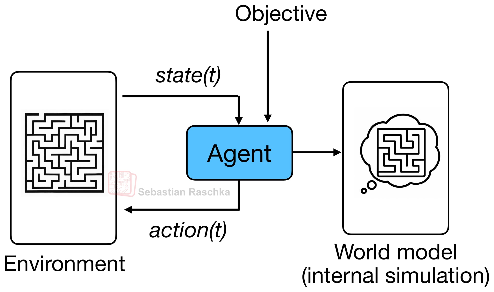
The term “world model”, as far as I know, was popularized by Ha and Schmidhuber’s 2018 paper of the same name: World Models, which used a VAE plus RNN architecture to learn an internal environment simulator for reinforcement learning agents. (But the term or concept itself essentially just refers to modeling a concept of a world or environment, so it goes back to reinforcement learning and robotics research in the 1980s.)

To be honest, I didn’t have the new interpretation of world models on my radar until Yann LeCun’s 2022 article A Path Towards Autonomous Machine Intelligence. It was essentially about mapping an alternative path to AI instead of LLMs.

That being said, world model papers were all focused on vision domains and spanned a wide range of architectures: from early VAE- and RNN-based models to transformers, diffusion models, and even Mamba-layer hybrids.

Now, as someone currently more focused on LLMs, the Code World Model paper (Sep 30, 2025) is the first paper to capture my full attention (no pun intended). This is the first world model (to my knowledge) that maps from text to text (or, more precisely, from code to code).

CWM is a 32-billion-parameter open-weight model with a 131k-token context window. Architecturally, it is still a dense decoder-only Transformer with sliding-window attention. Also, like other LLMs, it goes through pre-training, mid-training, supervised fine-tuning (SFT), and reinforcement learning stages, but the mid-training data introduces the world-modeling component.

So, how does this differ from a regular code LLM such as Qwen3-Coder?

Regular models like Qwen3-Coder are trained purely with next-token prediction. They learn patterns of syntax and logic to produce plausible code completions, which gives them a static text-level understanding of programming.

CWM, in contrast, learns to simulate what happens when the code runs. It is trained to predict the resulting program state, such as the value of a variable, after performing an action like modifying a line of code, as shown in the figure below.

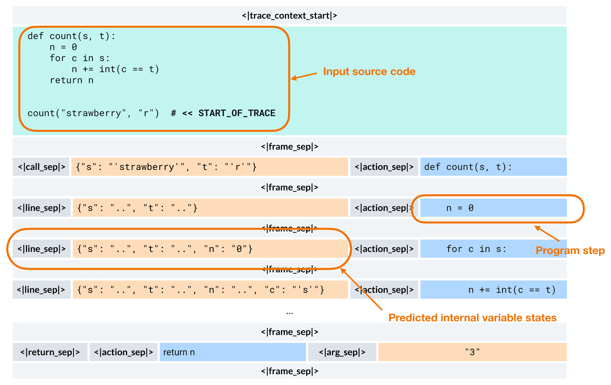
At inference time, CWM is still an autoregressive transformer that generates one token at a time, just like GPT-style models. The key difference is that these tokens can encode structured execution traces rather than plain text.

So, I would maybe not call it a world model, but a world model-augmented LLM.

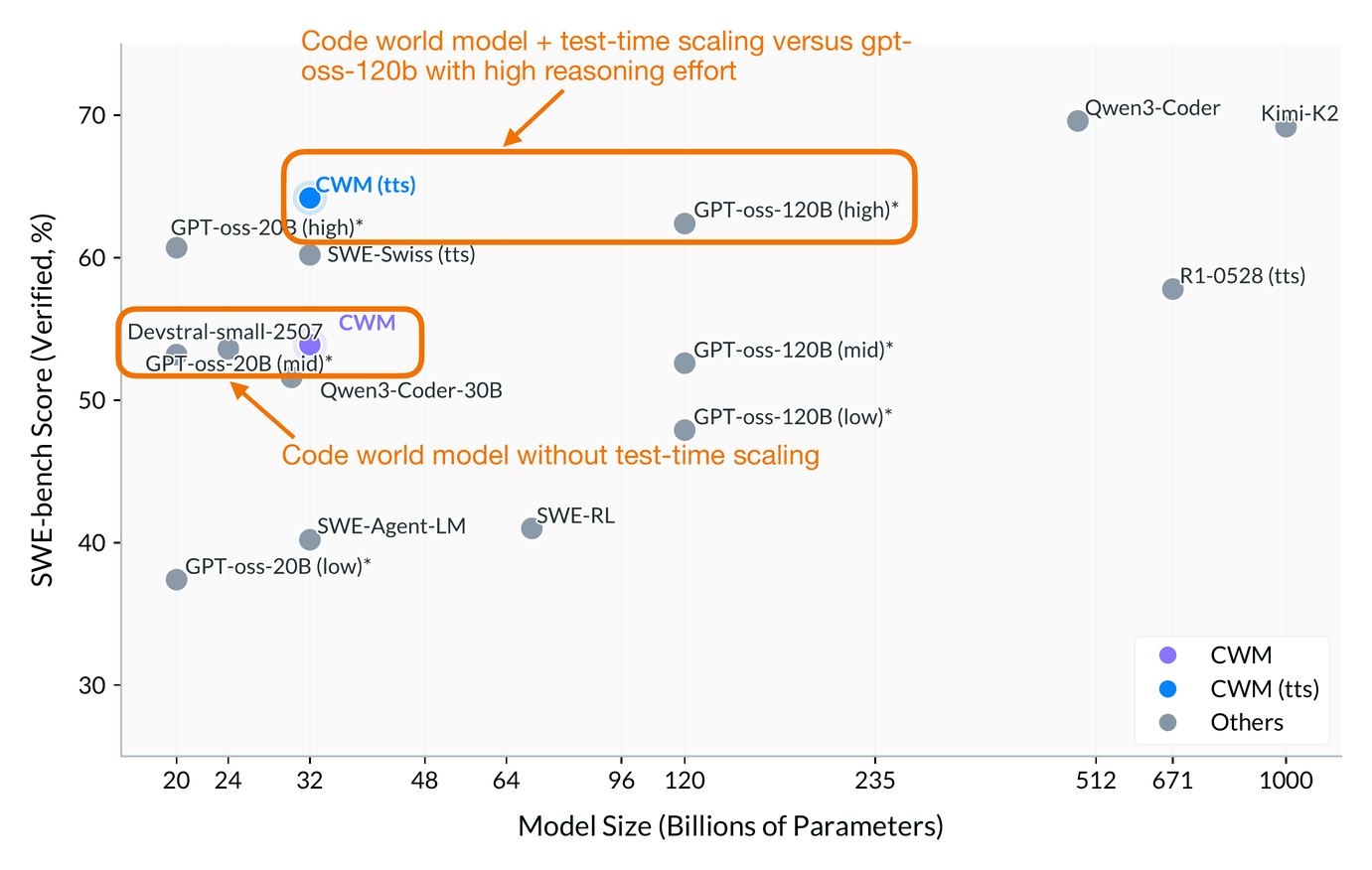
For a first attempt, it performs surprisingly well, and is on par with gpt-oss-20b (mid reasoning effort) at roughly the same size.

If test-time-scaling is used, it even performs slightly better than gpt-oss-120b (high reasoning effort) while being 4x smaller.

Note that their test-time scaling uses a best@k procedure with generated unit tests (think of a fancy majority voting scheme). It would have been interesting to see a tokens/sec or time-to-solution comparison between CWM and gpt-oss, as they use different test-time-scaling strategies (best@k versus more tokens per reasoning effort).

You may have noticed that all previous approaches still build on the transformer architecture. The topic of this last section does too, but in contrast to the models we discussed earlier, these are small, specialized transformers designed for reasoning.

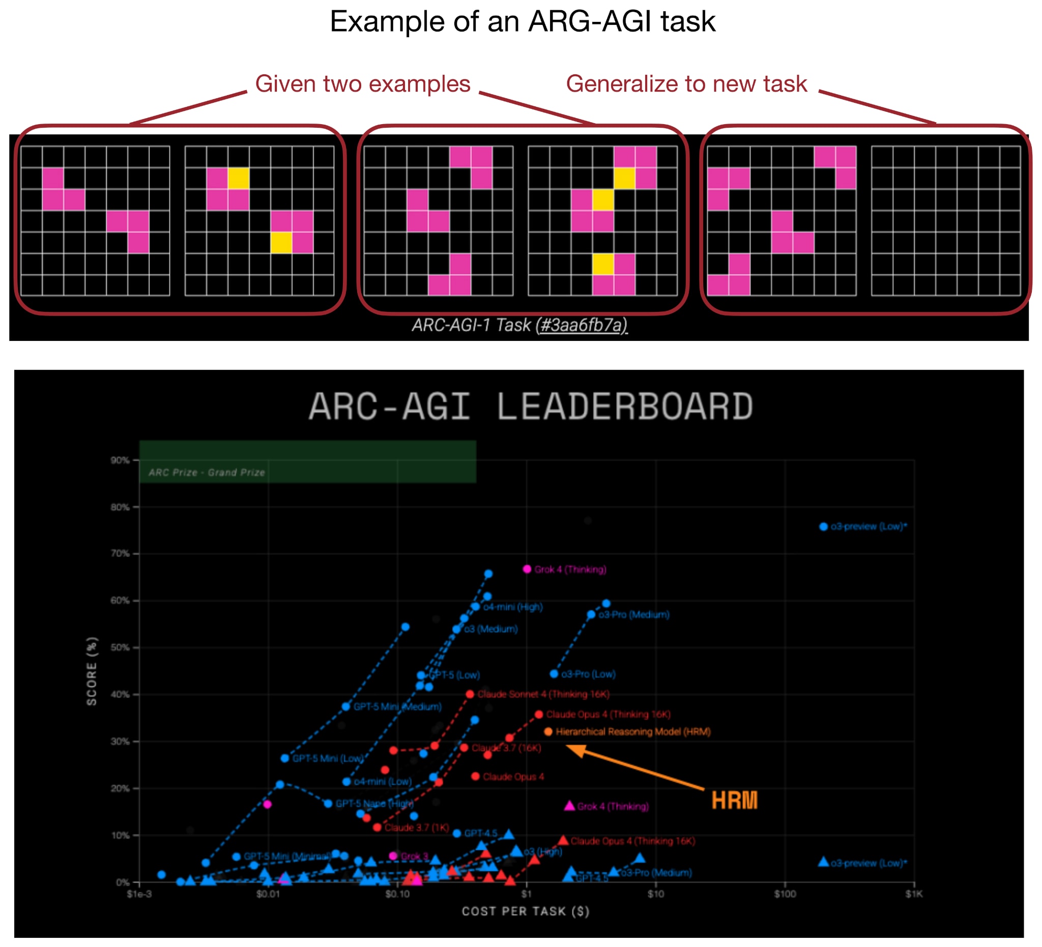
Yes, reasoning-focused architectures don’t always have to be large. In fact, with the Hierarchical Reasoning Model (HRM) a new approach to small recursive transformers has recently gained a lot of attention in the research community.

More specifically, the HRM developers showed that even very small transformer models (with only 4 blocks) can develop impressive reasoning capabilities (on specialized problems) when trained to refine their answers step by step. This resulted in a top spot on the ARC challenge.

The idea behind recursive models like HRM is that instead of producing an answer in one forward pass, the model repeatedly refines its own output in a recursive fashion. (As part of this process, each iteration refines a latent representation, which the authors see as the model’s “thought” or “reasoning” process.)

The first major example was HRM earlier in the summer, followed by the Mixture-of-Recursions (MoR) paper.

And most recently, Less is More: Recursive Reasoning with Tiny Networks (October 2025) proposes the Tiny Recursive Model (TRM, illustrated in the figure below), which is a simpler and even smaller model (7 million parameters, about 4× smaller than HRM) that performs even better on the ARC benchmark.

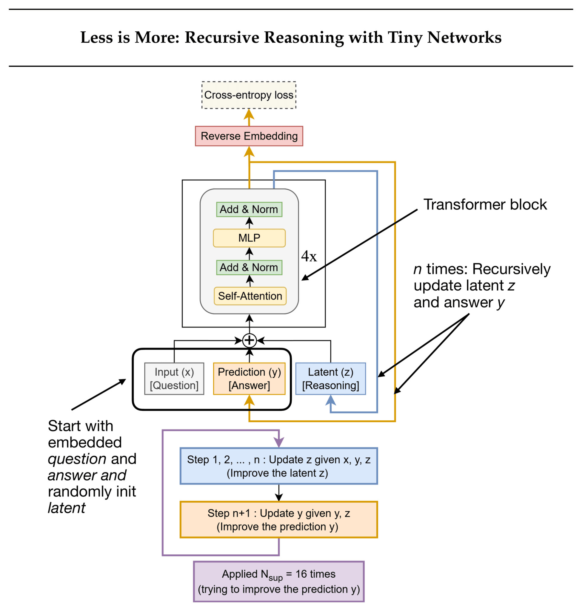
In the remainder of this section, let’s take a look at TRM in a bit more detail.

TRM refines its answer through two alternating updates:

1. It computes a latent reasoning state from the current question and answer.

2. It then updates the answer based on that latent state.

The training runs for up to 16 refinement steps per batch. Each step performs several no-grad loops to iteratively refine the answer. This is followed by a gradient loop that backpropagates through the full reasoning sequence to update the model weights.

It’s important to note that TRM is not a language model operating on text. However, because (a) it’s a transformer-based architecture, (b) reasoning is now a central focus in LLM research, and this model represents a distinctly different take on reasoning, and (c) many readers have asked me to cover HRM (and TRM is its more advanced successor) I decided to include it here.

While TRM could be extended to textual question-answer tasks in the future, TRM currently works on grid-based inputs and outputs. In other words, both the “question” and the “answer” are grids of discrete tokens (for example, 9×9 Sudoku or 30×30 ARC/Maze puzzles), not text sequences.

HRM consists of two small transformer modules (each 4 blocks) that communicate across recursion levels. TRM only uses a single 2-layer transformer. (Note that the previous TRM figure shows a 4× next to the transformer block, but that’s likely to make it easier to compare against HRM.)

TRM backpropagates through all recursive steps, whereas HRM only backpropagates through the final few.

HRM includes an explicit halting mechanism to determine when to stop iterating. TRM replaces this mechanism with a simple binary cross-entropy loss that learns when to stop iterating.

Performance-wise, TRM performs really well compared to HRM, as shown in the figure below.

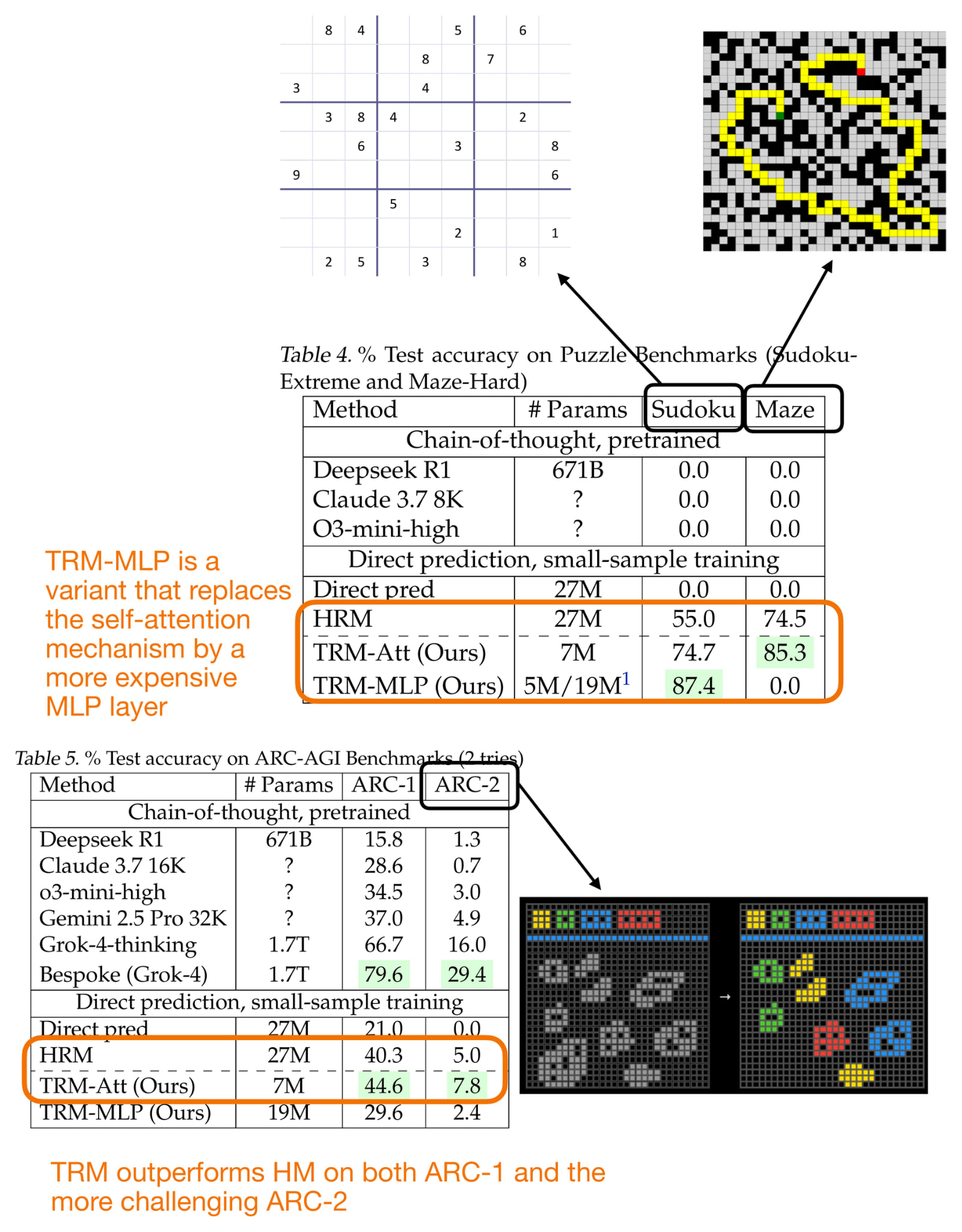
Figure 24: Performance comparison of the Hierarchical Reasoning Model (HRM) and Tiny Recursive Model (TRM).

The paper included a surprising number of ablation studies, which yielded some interesting additional insights. Here are two that stood out to me:

1. Fewer layers leads to better generalization. Reducing from 4 to 2 layers improved Sudoku accuracy from 79.5% to 87.4%.

2. Attention is not required. Replacing self-attention with a pure MLP layer also improved accuracy (74.7% to 87.4%). But this is only feasible here because the context is small and fixed-length.

While HRM and TRM achieve really good reasoning performance on these benchmarks, comparing them to large LLMs is not quite fair. HRM and TRM are specialized models for tasks like ARC, Sudoku, and Maze pathfinding, whereas LLMs are generalists. Sure, HRM and TRM can be adopted for other tasks as well, but they have to be specially trained on each task. So, in that sense, we can perhaps think of HRM and TRM as efficient pocket calculators, whereas LLM are more like computers, which can do a lot of other things as well.

Still, these recursive architectures are exciting proof-of-concepts that highlight how small, efficient models can “reason” through iterative self-refinement. Perhaps, in the future, such models could act as reasoning or planning modules embedded within larger tool-using LLM systems.

For now, LLMs remain ideal for broad tasks, but domain-specific recursive models like TRM can be developed to solve certain problems more efficiently once the target domain is well understood. Beyond the Sudoku, Maze finding, and ARC proof-of-concept benchmarks, there are possibly lots of use cases in the physics and biology domain where such models could find use.

As an interesting tidbit, the author shared that it took less than $500 to train this model, with 4 H100s for around 2 days. I am delighted to see that it’s still possible to do interesting work without a data center.

I originally planned to cover all models categories in the overview figure, but since the article ended up longer than I expected, I will have to save xLSTMs, Liquid Foundation Models, Transformer-RNN hybrids, and State Space Models for another time (although, Gated DeltaNet already gave a taste of State Space Models and recurrent designs.)

As a conclusion to this article, I want to repeat the earlier words, i.e., that standard autoregressive transformer LLMs are proven and have stood the test of time so far. They are also, if efficiency is not the main factor, the best we have for now.

Traditional Decoder-Style, Autoregressive Transformers

+ Proven & mature tooling
+ “well-understood”
+ Scaling laws
+ SOTA
- Expensive training
- Expensive inference (except for aforementioned tricks)

If I were to start a new LLM-based project today, autoregressive transformer-based LLMs would be my first choice.

I definitely find the upcoming attention hybrids very promising, which are especially interesting when working with longer contexts where efficiency is a main concern.

Linear Attention Hybrids

+ Same as decoder-style transformers
+ Cuts FLOPs/KV memory at long-context tasks
- Added complexity
- Trades a bit of accuracy for efficiency

On the more extreme end, text diffusion models are an interesting development. I’m still somewhat skeptical about how well they perform in everyday use, as I’ve only tried a few quick demos. Hopefully, we’ll soon see a large-scale production deployment with Google’s Gemini Diffusion that we can test on daily and coding tasks, and then find out how people actually feel about them.

Text Diffusion Models

+ Iterative denoising is a fresh idea for text
+ Better parallelism (no next-token dependence)
- Can’t stream answers
- Doesn’t benefit from CoT?
- Tricky tool-calling?
- Solid models but not SOTA

While the main selling point of text diffusion models is improved efficiency, code world models sit on the other end of the spectrum, where they aim to improve modeling performance. As of this writing, coding models, based on standard LLMs, are mostly improved through reasoning techniques, yet if you have tried them on trickier challenges, you have probably noticed that they (more or less) still fall short and can’t solve many of the trickier coding problems well.

I find code world models particularly interesting and believe they could be an important next step toward developing more capable coding systems.

Code World Model

+ Promising approach to improve code understanding
+ Verifiable intermediate states
- Inclusion of executable code traces complicates training
- Code running adds latency

Lastly, we covered small recursive transformers such as hierarchical and tiny reasoning models. These are super interesting proof-of-concept models. However, as of today, they are primarily puzzle solvers, not general text or coding models. So, they are not in the same category as the other non-standard LLM alternatives covered in this article. Nonetheless, they are very interesting proofs-of-concept, and I am glad researchers are working on them.

Right now, LLMs like GPT-5, DeepSeek R1, Kimi K2, and so forth are developed as special purpose models for free-form text, code, math problems and much more. They feel like brute-force and jack-of-all-trades approach that we use on a variety of tasks, from general knowledge questions to math and code.

However, when we perform the same task repeatedly, such brute-force approaches become inefficient and may not even be ideal in terms of specialization. This is where tiny recursive transformers become interesting: they could serve as lightweight, task-specific models that are both efficient and purpose-built for repeated or structured reasoning tasks.

Also, I can see them as potential “tools” for other tool-calling LLMs; for instance, when LLMs use Python or calculator APIs to solve math problems, special tiny reasoning models could fill this niche for other types of puzzle- or reasoning-like problems.

Small Recursive Transformers

+ Very small architecture
+ Good generalization on puzzles
- Special purpose models
- Limited to puzzles (so far)

This has been a long article, but I hope you discovered some of the fascinating approaches that often stay outside the spotlight of mainstream LLMs.

And if you’ve been feeling a bit bored by the more or less conventional LLM releases, I hope this helped rekindle your excitement about AI again because there’s a lot of interesting work happening right now!

This magazine is a personal passion project, and your support helps keep it alive.

If you’d like to support my work, please consider my Build a Large Language Model (From Scratch) book or its follow-up, Build a Reasoning Model (From Scratch). (I’m confident you’ll get a lot out of these; they explain how LLMs work in depth you won’t find elsewhere.)

Thanks for reading, and for helping support independent research!

If you read the book and have a few minutes to spare, I’d really appreciate a brief review. It helps us authors a lot!

Your support means a great deal! Thank you!