A simple search engine from scratch

4 days ago 1

*if you include word2vec.

Chris and I spent a couple hours the other day creating a search engine for my blog from “scratch”. Mostly he walked me through it because I only vaguely knew what word2vec was before this experiment.

The search engine we made is built on word embeddings. This refers to some function that takes a word and maps it onto N-dimensional space (in this case, N=300) where each dimension vaguely corresponds to some axis of meaning. Word2vec from Scratch is a nice blog post that shows how to train your own mini word2vec and explains the internals.

The idea behind the search engine is to embed each of my posts into this domain by adding up the embeddings for the words in the post. For a given search, we’ll embed the search the same way. Then we can rank all posts by their cosine similarities to the query.

The equation below might look scary but it’s saying that the cosine similarity, which is the cosine of the angle between the two vectors cos(theta), is defined as the dot product divided by the product of the magnitudes of each vector. We’ll walk through it all in detail.

Equation from Wikimedia's Cosine similarity page.

Cosine distance is probably the simplest method for comparing a query embedding to document embeddings to rank documents. Another intuitive choice might be euclidean distance, which would measure how far apart two vectors are in space (rather than the angle between them).

We prefer cosine distance because it preserves our intuition that two vectors have similar meanings if they have the same proportion of each embedding dimension. If you have two vectors that point in the same direction, but one is very long and one very short, these should be considered the same meaning. (If two documents are about cats, but one says the word cat much more, they’re still just both about cats).

Let’s open up word2vec and embed our first words.

Embedding

We take for granted this database of the top 10,000 most popular word embeddings, which is a 12MB pickle file that vaguely looks like this:

couch [0.23, 0.05, ..., 0.10] banana [0.01, 0.80, ..., 0.20] ...

Chris sent it to me over the internet. If you unpickle it, it’s actually a NumPy data structure: a dictionary mapping strings to numpy.float32 arrays. I wrote a script to transform this pickle file into plain old Python floats and lists because I wanted to do this all by hand.

The loading code is straighforward: use the pickle library. The usual security caveats apply, but I trust Chris.

import pickle def load_data(path): with open(path, "rb") as f: return pickle.load(f) word2vec = load_data("word2vec.pkl")

You can print out word2vec if you like, but it’s going to be a lot of output. I learned that the hard way. Maybe print word2vec["cat"] instead. That will print out the embedding.

To embed a word, we need only look it up in the enormous dictionary. A nonsense or uncommon word might not be in there, though, so we return None in that case instead of raising an error.

def embed_word(word2vec, word): return word2vec.get(word)

To embed multiple words, we embed each one individually and then add up the embeddings pairwise. If a given word is not embeddable, ignore it. It’s only a problem if we can’t understand any of the words.

def vec_add(a, b): return [x + y for x, y in zip(a, b)] def embed_words(word2vec, words): result = [0.0] * len(next(iter(word2vec.values()))) num_known = 0 for word in words: embedding = word2vec.get(word) if embedding is not None: result = vec_add(result, embedding) num_known += 1 if not num_known: raise SyntaxError(f"I can't understand any of {words}") return result

That’s the basics of embedding: it’s a dictionary lookup and vector adds.

embed_words([a, b]) == vec_add(embed_word(a), embed_word(b))

Now let’s make our “search engine index”, or the embeddings for all of my posts.

Embedding all of the posts

Embedding all of the posts is a recursive directory traversal where we build up a dictionary mapping path name to embedding.

import os def load_post(pathname): with open(pathname, "r") as f: contents = f.read() return normalize_text(contents).split() def load_posts(): # Walk _posts looking for *.md files posts = {} for root, dirs, files in os.walk("_posts"): for file in files: if file.endswith(".md"): pathname = os.path.join(root, file) posts[pathname] = load_post(pathname) return posts post_embeddings = {pathname: embed_words(word2vec, words) for pathname, words in posts.items()} with open("post_embeddings.pkl", "wb") as f: pickle.dump(post_embeddings, f)

We do this other thing, though: normalize_text. This is because blog posts are messy and contain punctuation, capital letters, and all other kinds of nonsense. In order to get the best match, we want to put things like “CoMpIlEr” and “compiler” in the same bucket.

import re def normalize_text(text): return re.sub(r"[^a-zA-Z]", r" ", text).lower()

We’ll do the same thing for each query, too. Speaking of, we should test this out. Let’s make a little search REPL.

A little search REPL

We’ll start off by using some Python’s built-in REPL creator library, code. We can make a subclass that defines a runsource method. All it really needs to do is process the source input and return a falsy value (otherwise it waits for more input).

import code class SearchRepl(code.InteractiveConsole): def __init__(self, word2vec, post_embeddings): super().__init__() self.word2vec = word2vec self.post_embeddings = post_embeddings def runsource(self, source, filename="<input>", symbol="single"): for result in self.search(source): print(result)

Then we can define a search function that pulls together our existing functions. Just like that, we have a search:

class SearchRepl(code.InteractiveConsole): # ... def search(self, query_text, n=5): # Embed query words = normalize_text(query_text).split() try: query_embedding = embed_words(self.word2vec, words) except SyntaxError as e: print(e) return # Cosine similarity post_ranks = {pathname: vec_cosine_similarity(query_embedding, embedding) for pathname, embedding in self.post_embeddings.items()} posts_by_rank = sorted(post_ranks.items(), reverse=True, key=lambda entry: entry[1]) top_n_posts_by_rank = posts_by_rank[:n] return [path for path, _ in top_n_posts_by_rank]

Yes, we have to do a cosine similarity. Thankfully, the Wikipedia math snippet translates almost 1:1 to Python code:

import math def vec_norm(v): return math.sqrt(sum([x*x for x in v])) def vec_cosine_similarity(a, b): assert len(a) == len(b) a_norm = vec_norm(a) b_norm = vec_norm(b) dot_product = sum([ax*bx for ax, bx in zip(a, b)]) return dot_product/(a_norm*b_norm)

Finally, we can create and run the REPL.

sys.ps1 = "QUERY. " sys.ps2 = "...... " repl = SearchRepl(word2vec, post_embeddings) repl.interact(banner="", exitmsg="")

This is what interacting with it looks like:

QUERY. type inference _posts/2024-10-15-type-inference.md _posts/2025-03-10-lattice-bitset.md _posts/2025-02-24-sctp.md _posts/2022-11-07-inline-caches-in-skybison.md _posts/2021-01-14-inline-caching.md QUERY.

This is a sample query from a very small dataset (my blog). It’s a pretty good search result, but it’s probably not representative of the overall search quality. Chris says that I should cherry-pick “because everyone in AI does”.

Okay, that’s really neat. But most people who want to look for something on my website do not run for their terminals. Though my site is expressly designed to work well in terminal browsers such as Lynx, most people are already in a graphical web browser. So let’s make a search front-end.

A little web search

So far we’ve been running from my local machine where I don’t mind having a 12MB file of weights sitting around. Now that we’re moving to web, I would rather not burden casual browsers with an unexpected big download. So we need to get clever.

Fortunately, Chris and I had both seen this really cool blog post that talks about hosting a SQLite database on GitHub Pages. The blog post details how the author:

compiled SQLite to Wasm so it could run on the client,
built a virtual filesystem so it could read database files from the web,
did some smart page fetching using the existing SQLite indexes,
built additional software to fetch only small chunks of the database using HTTP Range requests

That’s super cool, but again: SQLite, though small, is comparatively big for this project. We want to build things from scratch. Fortunately, we can emulate the main ideas.

We can give the word2vec dict a stable order and split it into two files. One file can just have the embeddings, no names. Another file, the index, can map every word to the byte start and byte length of the weights for that word (we figure start&length is probably smaller on the wire than start&end).

# vecs.jsonl [0.23, 0.05, ..., 0.10] [0.01, 0.80, ..., 0.20] ...

# index.json {"couch": [0, 20], "banana": [20, 30], ...}

The cool thing about this is that index.json is dramatically smaller than the word2vec blob, weighing in at 244KB. Since that won’t change very often (how often does word2vec change?), I don’t feel so bad about users eagerly downloading the entire index. Similarly, the post_embeddings.json is only 388KB. They’re even cacheable. And automagically (de)compressed by the server and browser (to 84KB and 140KB, respectively). Both would be smaller if we chose a binary format, but we’re punting on that for the purposes of this post.

Then we can make HTTP Range requests to the server and only download the parts of the weights that we need. It’s even possible to bundle all of the ranges into one request (it’s called multipart range). Unfortunately, GitHub Pages does not appear to support multipart, so instead we download each word’s range in a separate request.

Here’s the pertinent JS code, with (short, very familiar) vector functions omitted:

(async function() { // Download stuff async function get_index() { const req = await fetch("index.json"); return req.json(); } async function get_post_embeddings() { const req = await fetch("post_embeddings.json"); return req.json(); } const index = new Map(Object.entries(await get_index())); const post_embeddings = new Map(Object.entries(await get_post_embeddings())); // Add search handler search.addEventListener("input", debounce(async function(value) { const query = search.value; // TODO(max): Normalize query const words = query.split(/\s+/); if (words.length === 0) { // No words return; } const requests = words.reduce((acc, word) => { const entry = index.get(word); if (entry === undefined) { // Word is not valid; skip it return acc; } const [start, length] = entry; const end = start+length-1; acc.push(fetch("vecs.jsonl", { headers: new Headers({ "Range": `bytes=${start}-${end}`, }), })); return acc; }, []); if (requests.length === 0) { // None are valid words :( search_results.innerHTML = "No results :("; return; } const responses = await Promise.all(requests); const embeddings = await Promise.all(responses.map(r => r.json())); const query_embedding = embeddings.reduce((acc, e) => vec_add(acc, e)); const post_ranks = {}; for (const [path, embedding] of post_embeddings) { post_ranks[path] = vec_cosine_similarity(embedding, query_embedding); } const sorted_ranks = Object.entries(post_ranks).sort(function(a, b) { // Decreasing return b[1]-a[1]; }); // Fun fact: HTML elements with an `id` attribute are accessible as JS // globals by that same name. search_results.innerHTML = ""; for (let i = 0; i < 5; i++) { search_results.innerHTML += `<li>${sorted_ranks[i][0]}</li>`; } })); })();

You can take a look at the live search page. In particular, open up the network requests tab of your browser’s console. Marvel as it only downloads a couple 4KB chunks of embeddings.

So how well does our search technology work? Let’s try to build an objective-ish evaluation.

Evaluation

We’ll design a metric that roughly tells us when our search engine is better or worse than a naive approach without word embeddings.

We start by collecting an evaluation dataset of (document, query) pairs. Right from the start we’re going to bias this evaluation by collecting this dataset ourselves, but hopefully it’ll still help us get an intuition about the quality of the search. A query in this case is just a few search terms that we think should retrieve a document successfully.

sample_documents = { "_posts/2024-10-27-on-the-universal-relation.md": "database relation universal tuple function", "_posts/2024-08-25-precedence-printing.md": "operator precedence pretty print parenthesis", "_posts/2019-03-11-understanding-the-100-prisoners-problem.md": "probability strategy game visualization simulation", # ... }

Now that we’ve collected our dataset, let’s implement a top-k accuracy metric. This metric measures the percentage of the time a document appears in the top k search results given its corresponding query.

def compute_top_k_accuracy( # Mapping of post to sample search query (already normalized) # See sample_documents above eval_set: dict[str, str], max_n_keywords: int, max_top_k: int, n_query_samples: int, ) -> list[list[float]]: counts = [[0] * max_top_k for _ in range(max_n_keywords)] for n_keywords in range(1, max_n_keywords + 1): for post_id, keywords_str in eval_set.items(): for _ in range(n_query_samples): # Construct a search query by sampling keywords keywords = keywords_str.split(" ") sampled_keywords = random.choices(keywords, k=n_keywords) query = " ".join(sampled_keywords) # Determine the rank of the target post in the search results ids = search(query, n=max_top_k) rank = safe_index(ids, post_id) # Increment the count of the rank if rank is not None and rank < max_top_k: counts[n_keywords - 1][rank] += 1 accuracies = [[0.0] * max_top_k for _ in range(max_n_keywords)] for i in range(max_n_keywords): for j in range(max_top_k): # Divide by the number of samples to get the average across samples and # divide by the size of the eval set to get accuracy over all posts. accuracies[i][j] = counts[i][j] / n_query_samples / len(eval_set) # Accumulate accuracies because if a post is retrieved at rank i, # it was also successfully retrieved at all ranks j > i. if j > 0: accuracies[i][j] += accuracies[i][j - 1] return accuracies

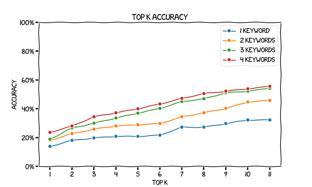
Let’s start by evaluating a baseline search engine. This implementation doesn’t use word embeddings at all. We just normalize the text, and count the number of times each query word occur in the document, then rank the documents by number of query word occurrences. Plotting top-k accuracy for various values of k gives us the following chart. Note that we get higher accuracy as we increase k – in the limit, as k approaches our number of documents we approach 100% accuracy.

You also might notice that the accuracy increases as we increase the number of keywords. We can see also the lines getting closer together as the number of keywords increases, which indicates there are diminishing marginal returns for each new keyword.

Do these megabytes of word embeddings actually do anything to improve our search? We would have to compare to a baseline. Maybe that baseline is adding up the counts of all keywords in each document to rank them. We leave this as an exercise to the reader because we ran out of time :)

It would also be interesting to see how a bigger word2vec helps accuracy. While sampling for top-k, there is a lot of error output (I can't understand any of ['prank', ...]). These unknown words get dropped from the search. A bigger word2vec (more than 10,000 words) might contain these less-common words and therefore search better.

Wrapping up

You can build a small search engine from “scratch” with only a hundred or so lines of code. See the full search.py, which includes some of the extras for evaluation and plotting.

Future ideas

We can get fancier than simple cosine similarity. Let’s imagine that all of our documents talk about computers, but only one of them talks about compilers (wouldn’t that be sad). If one of our search terms is “computer” that doesn’t really help narrow down the search and is noise in our embeddings. To reduce noise we can employ a technique called TF-IDF (term frequency inverse document frequency) where we factor out common words across documents and pay closer attention to words that are more unique to each document.

Read Entire Article