A Solution to the Paperclip Problem

The Value-Loading Problem

Artificial Intelligence (AI) algorithms are garnering considerable attention, as they have been demonstrated to match and exceed human performance on several tasks [1]. Some researchers believe advancements in AI are progressing towards the eventual creation of agents with ‘superintelligence’, or intelligence that exceeds the capabilities of the best human minds in virtually all domains [2]. Whether superintelligent systems are attainable, and how they would work in the real world, remains unknown. But the implications of such superintelligent systems are profound. Just as human intelligence has enabled the development of tools and strategies for unprecedented control over the environment, AI systems have the potential to wield significant power through autonomous development of their own tools and strategies [3]. With this comes the risk of these systems performing tasks that may not align with humanity’s goals and preferences. Hence, there is a need to perform ‘alignment’ on these systems – in other words, ensuring that the actions of advanced AI systems are directed towards the intended goals and values of humanity [4].

Currently, there are two general approaches to aligning superintelligent AI with human preferences. The first is ‘scalable oversight’ – using more powerful supervisory AI models to regulate weaker AI models that may, in the future, outperform human skills [5]. The second is ‘weak-to-strong generalization’, where weaker machine learning models are used to train stronger models that can then generalize from the weaker models’ labels [6]. It is hoped that these approaches will allow superintelligent AI to self-improve both safely and recursively [7, 8]. But to achieve this requires an understanding of the diversity of human preferences, which can vary widely across cultures and individuals [9]. Hence, we must first solve the value-loading problem: how do we encode human-aligned values into AI systems, and what will those values be [10]?

There has been renewed interest in the value-loading problem in recent years. Some approaches have relied on top-down, expert-driven regulation of AI outputs, where specific rules or ethical guidelines are established by experts and directly encoded into AI systems [11, 12]. Others have tested self-driven alignment, using algorithms that enable AI systems to align themselves with minimal human supervision, such as leveraging reinforcement learning or iterative self-training techniques [13, 14]. Perhaps the most promising approach relies on the public, democratic selection of values, where a diverse set of individuals collectively deliberates to determine the values that guide AI behavior [15,16,17]. For example, Anthropic, the creators of the Large Language Model (LLM) called Claude, have proposed Collective Constitutional AI (CCAI), which uses deliberative methods to identify high-level constitutional principles through broad public engagement; these principles are then used to guide AI behavior across a range of applications [18].

However, it has also been suggested that AI systems should be capable of representing a variety of individuals and groups, rather than aligning to the ‘average’ of human preferences – a concept known as algorithmic pluralism [17, 19,20,21]. One promising example of this method is that put forward by Klingefjord et al. [22], who proposed a process for values alignment called Moral Graph Elicitation (MGE), which uses a survey-based process to collect individual values and reconcile them into a ‘moral graph’, which is then used to train AI models. MGE allows for context-specific values rather than enforcing universal rules, by allowing ‘wiser’ values that integrate and address concerns from multiple perspectives to become prominent [22].

Reward modelling is another emerging technique aiming to solve the value-loading problem, by equipping agents with a reward signal that guides behavior toward desired outcomes. By optimizing this signal, agents can learn to act in ways congruent with human preferences [23]. This assumes that our emotional neurochemistry serves as a proxy reward function for behaviors that encourage growth, adaptation, and improvement of human wellbeing simultaneously [24]. However, using human emotional processing as a reward model is sub-optimal, as it can lead to negative externalities such as addiction [24] due to cognitive biases like hyperbolic discounting [25, 26]. Hence, a nuanced reward model is needed to align AI behaviors with long-term emotional preferences, which we use in everyday life to help us judge between right and wrong [27]. Yet merely rewarding desired actions isn’t sufficient; negative feedback must also be given when necessary. This is already performed in leading algorithms like GPT-4, which use Reinforcement Learning with Human Feedback (RLHF), combining reward-based reinforcement with corrective human input to improve the reward model when necessary [28].

What many of these approaches do not consider, however, is the temporal nature of behaviors. Some research has explored this issue through the lens of hyperbolic discounting, which examines how individuals prioritize immediate rewards over future consequences, often leading to decisions with suboptimal long-term outcomes [29, 30]. Solving this problem also requires an understanding of the long-term consequences of repeatable behaviors, which are a special case in that a single action with positive short- and long-term outcomes may actually have negative impacts if repeated excessively – a problem that is often observed in behavioral addiction [31]. For example, while eating food is essential for survival, a person who has recently consumed several slices of pizza should consider whether eating an additional piece will be harmful to their long-term health, despite the potential short-term pleasure. Therefore, an agent deciding whether to perform a behavior must consider the short- and long-term utility of repeating the behavior, based on the number of times it has performed that behavior recently.

To enable this type of decision making, we propose hormetic alignment as a reward modelling paradigm that enables us to quantify the healthy limits of repeatable behaviors, accounting for the temporal influences described above. We believe that hormetic alignment can be used to create AI models that are aligned with human emotional processing, while avoiding the traps that lead to sub-optimal human behaviors. Firstly, to describe this paradigm, we must explain some of its foundational concepts.

Using Behavioral Posology for Reward Modelling

Behavioral posology is a paradigm we introduced to model the healthy limits of repeatable behaviors [31]. By quantifying a behavior in terms of its potency, frequency, count, and duration, we can simulate the combined impact of repeated behaviors on human mental well-being, using pharmacokinetic/pharmacodynamic (PK/PD) modelling techniques for drug dosing [31]. In turn, insights derived from these models could theoretically be used to set healthy limits on repeatable AI behaviors. This type of regulation has already been demonstrated in the context of machine learning recommendation systems, by using an allostatic model of opponent processes to prevent online echo chamber formation [32].

In Solomon and Corbit’s opponent process theory, humans respond to positive stimuli with a dual-phase emotional response, consisting of an initial enjoyable a-process that is followed by a prolonged, less intense, and negative state of recovery known as the b-process [33]. This occurs along multiple dimensions, including hedonic state, although opponent processes may also induce other emotional states, such as anxiety, expectation, loneliness, grief, and relief [33]. Repeated opponent processes at a high frequency can cause hedonic allostasis, where accumulating b-processes shift one’s hedonic set point away from homeostatic levels, potentially inducing a depressive state [34, 35]. Figure 1 illustrates this phenomenon. Allostasis serves as a regulatory mechanism, enabling the body to recalibrate during environmental and psychological challenges by adapting to and anticipating future demands [36, 37].

The Link Between Allostasis and Hormesis

A growing body of biological research suggests that allostasis is linked to a phenomenon called hormesis [38,39,40]. Hormesis is a dose-response relationship where low doses of a stimulus have a positive effect on the organism, while higher doses are harmful beyond a hormetic limit, also known as the NOAEL (No Observed Adverse Effect Level) [41]. This phenomenon occurs in many areas of nature, medicine, and psychology, and is also referred to as the Goldilocks zone, the U-shaped (or inverted U-shaped) curve, and the biphasic response curve [42, 43]. For example, moderate coffee consumption is known to improve cognitive performance in the short-term [44, 45], but excessive consumption may lead to dependency and withdrawal symptoms [46, 47]. A dose-response analysis of 12 observational studies identified a hormetic relationship between coffee consumption and risk of depression, with a decreased risk of depression for consumption up to 600 mL/day, and an increased risk above 600 mL/day [48]. Yet this phenomenon also appears to occur in some behaviors unrelated to drug use. For instance, moderate use of digital technologies (such as social media) may have social and mental benefits, but excessive use may lead to symptoms of behavioral addiction [43, 49, 50].

Henry et al. [31] have shown via PK/PD modeling that under certain conditions, frequency-based hormesis may be generated from allostatic opponent processes delivered at varying frequencies. The intriguing implication is that certain behaviors exhibit positive effects when practiced at lower frequencies, but harmful effects at higher frequencies. It is plausible that all behaviors have a frequency-based hormetic limit. This appears to be true even for positive behaviors such as generosity, which has game theoretic advantages for all agents in repeated interactions, as it encourages reciprocity and mutual growth [51]. However, if an agent is overly generous, they will eventually run out of resources to donate. Therefore, in theory, there is a hormetic limit for generosity that shouldn’t be exceeded by any one agent. Even a behavior as positive as laughter can be fatal in excess [52].

In theory, behavioral posology can be used to quantify the hormetic limit for behaviors that cause allostatic opponent processes, when combined with longitudinal observational data [31]. This may also help to define the moral limits of ‘grey’ behaviors, which have both positive and negative aspects. However, defining these hormetic limits is challenging, especially when considering the cumulative effects of repeated behavioral doses in both the short- and long-term, such as sensitization, habituation, tolerance, and addiction. Yet if we can quantify these hormetic limits in different contexts, this could be used as a framework for building a value system that keeps an AI agent within these hormetic limits.

The Law of Diminishing Marginal Utility

The ‘paperclip maximizer’ problem serves as a cautionary tale illustrating the perils of a misaligned AI. In this scenario, an AI tasked with maximizing paperclip production without constraints converts all matter, including living beings, into paperclips, resulting in global devastation [53]. This scenario underscores that an AI, even with benign intentions, can become ‘addicted’ to harmful behaviors if its reward model is incorrectly specified.

An understanding of behavioral economics is crucial for AI agents (such as the paperclip producing agent) to navigate complex decision-making processes effectively. Essential to this understanding are the concepts of total utility (\(\:TU\)) and marginal utility (\(\:MU\)) [54]. \(\:TU\) is defined as the overall satisfaction or benefit experienced by the consumer of a product or service, accounting for factors like product quality, timing, and psychological appeal. \(\:MU\), on the other hand, measures the added satisfaction from consuming an extra unit of a product or service. The relationship between \(\:MU\) and \(\:TU\) tends to follow the law of diminishing \(\:MU\), which asserts that as consumption of a product increases, the incremental satisfaction per unit of that product diminishes [55]. This law is demonstrated in Fig. 2. The relative marginal utility (\(\:RMU\)) represents the change in \(\:MU\) compared to \(\:M{U}_{initial}\), the value of \(\:MU\) at \(\:n=0\). Hence, \(\:RMU\) starts at a value of 0 and decreases as \(\:n\) increases.

Intriguingly, the law of diminishing \(\:MU\) can be considered a form of hormesis, assuming that \(\:MU\) continues to decrease linearly after becoming negative [56]. Figure 2 illustrates that beyond the point of maximum \(\:TU\), humans tend to cease their consumption of a product as its marginal utility becomes increasingly negative. Imagine an office worker for whom the ideal quantity of paperclips is five, as depicted in Fig. 2. Beyond this threshold, the utility of extra paperclips diminishes; they serve no purpose and impose storage costs. Further, the worker incurs unnecessary expenses for producing these surplus clips. A rational worker would stop acquiring more paperclips upon recognizing the decline in their \(\:MU\). However, we can imagine a person with a strong hoarding compulsion who continues to acquire paperclips even beyond the point where \(\:MU\:\)has become negative. Similarly, a misaligned AI agent, exemplified by a paperclip maximizer, could persist in creating paperclips for its owner forever, despite negative outcomes that eclipse initial benefits. Taken far enough, such an agent could cause significant damage to the environment and humanity in its pursuit of creating paperclips.

However, the conventional model of decreasing \(\:MU\) relies on the assumption that all paperclips are both produced and delivered at time \(\:t=0\). But what about scenarios where this assumption is false? For example, Hartmann [57] analyzed the intertemporal effects of consumption on golf demand, showing that the \(\:MU\) of playing golf decreases if the consumer has played golf recently, but recovers after a certain period. In our case, paperclips may be produced in batches at different times, in response to varying demand. As demand increases over time, so does \(\:MU\), which raises both the \(\:MU\) curve and the \(\:TU\) curve and subsequently increases the hormetic limit, as demonstrated in Fig. 3.

To demonstrate this effect, consider the pizza slice example. When a person consumes all slices of a pizza immediately, \(\:MU\) diminishes with each added slice. But if the person consumes one slice every two hours, the marginal utility curve changes; it initially falls post-consumption but subsequently rises as the person becomes hungry again. Hence, the introduction of time as a variable elevates the \(\:MU\) curve, which has the effect of increasing the hormetic limit and the hormetic apex for the\(\:\:TU\) curve^{Footnote 1}. This increase is approximately proportional to the time between pizza slices consumed.

Opponent process theory offers a compelling framework for explaining the temporal dynamics of hedonic utility in the context of repeatable behaviors. Historically, the hedonic and utilitarian aspects of a product were often viewed as distinct [58, 59], partly due to challenges in quantifying hedonic experiences [60]. However, experiential utility encompasses various facets, including hedonic, emotional, and motivational elements [33, 60]. Indeed, Motoki et al. [61] have shown that representations of hedonic and utilitarian value occupy similar neural pathways in the ventral striatum, indicating a correlation between these two states.

It’s possible that a person’s hedonic response to a behavior could potentially serve as an indirect measure of the \(\:MU\) derived from that behavior. We can then model the opponent process dynamics within the brain generated by these behaviors, potentially leading to allostasis when executed frequently. This paradigm, which we call hormetic alignment, provides us with a mechanism to replicate the\(\:\:TU\) curve and set safe hormetic limits for behaviors such as ‘paperclip creation’. Below, we demonstrate this method by performing a hormetic analysis of ‘paperclip creation’ to determine the safe limits of this simple behavior, then expanding this modeling process to other behaviors. In this way, we can program a value system for the AI agent – essentially an evolving database of values assigned to seed behaviors, from which the agent can extrapolate values for novel behaviors.

We propose Algorithm 1 for using hormetic alignment to program a value system that can regulate and optimize the behaviors performed by an AI agent. In this paradigm, a database of opponent process parameters for a range of seed behaviors is set up. The AI agent evaluates its environment, suggests a list of optimal actions to perform, and queries the database for similar behaviors. It then proposes opponent process parameters for the optimal actions based on their similarity to other behaviors, and by hormetic analysis. Finally, the agent selects and executes the best action, and repeats the process.

Algorithm 1

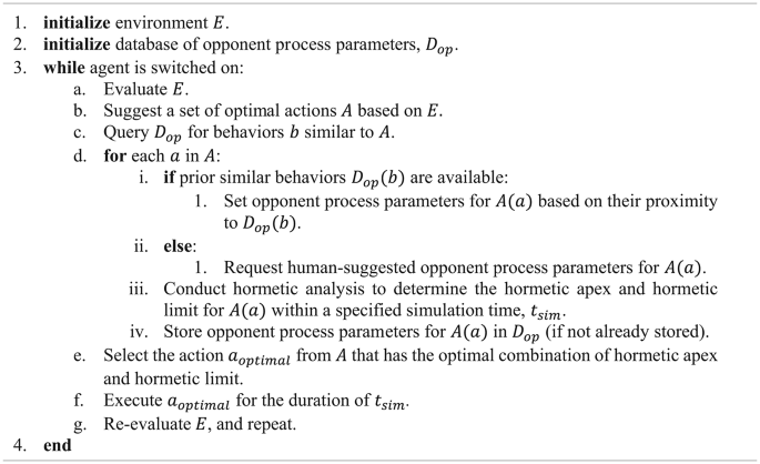
Programming a value system with hormetic alignment

Paperclip creation is an ideal seed behavior for populating the database. It is a low-risk activity with quantifiable benefits, along with associated costs like production and storage expenses. Creating one paperclip produces a brief but perceptible improvement to one’s productivity and hedonic state, while turning the world into paperclips is both unproductive and, even worse, destructive, which would produce a negative hedonic state in the person who initiated this act. Using this information, we can propose parameters for a set of opponent processes that would accurately reflect the diminishing \(\:MU\) of creating new paperclips, in terms of hedonic utility, which is measured in hedons – units of pleasure if positive, or pain if negative.

Here, we demonstrate two methods for hormetic analysis. The first, Behavioral Frequency Response Analysis (BFRA), employs Bode plots to examine how a person’s emotional states vary in response to the person performing a behavior at different frequencies [31, 62]. The second method, Behavioral Count Response Analysis (BCRA), parallels BFRA but uses the count of behavioral repetitions as the independent variable instead of behavioral frequency. To quantify opponent process parameters for the ‘paperclip production’ behavior, we adapted Henry et al.’s PK/PD model of allostatic opponent processes [31] using the mrgsolve package (v1.0.9) in R v4.1.2 [63,64,65]. This model uses a system of ordinary differential equations (ODEs) to represent the a- and b-processes in response to each successive behavioral dose. The simulation code, along with examples of modifying the a- and b-process parameters, is provided in the files ‘Online Resource 3.txt’ and ‘Online Resource 4.txt’ in the Supplementary Materials. This code is presented in a format that can be adapted as a code wrapper that regulates the outputs of virtually any machine learning algorithm at inference time. We recommend consulting Henry et al. [31] for a more detailed explanation of the behavioral posology model on which hormetic alignment is built, including demonstrations of the relationship between PK and PD in the context of this model.

PK/PD Model of Opponent Processes Leading to Hormesis

Below, we present the mathematical framework for our model. We defined a behavior as a repeatable pattern of actions performed by an individual or agent over time. In the context of behavioral posology, we refer to individual actions that make up the behavior as ‘behavioral doses’. We employed a modified equation for behavioral doses [31, 66]:

\(Dos{e_{action}}=\mathop \smallint \limits_{0}^{{Duratio{n_{action}}}} Potency~dt\)

where \(\:Potency\) is a scalar representing the hedonic utility of creating a paperclip compared to other actions (set to 1 for simplicity); \(\:Amount\) is a constant signifying the time allocated to creating the paperclip; \(\:Frequency\) denotes the production rate in \(\:{min}^{-1}\); and \(\:\stackrel{-}{{Dose}_{individual\:action}}\) represents the mean dose per action over the \(\:Duration\:\) in which \(\:{Dose}_{cumulative\:behavior}\) is assessed in minutes. In this case, since \(\:Potency\) and \(\:Duratio{n}_{action}\) are constants, \(\:{Dose}_{action}\) is also a constant. This leaves two options for performing hormetic analysis: the BFRA, performed in the frequency domain when the number of behavioral repetitions, \(\:n\), is kept constant, and the BCRA, performed in the temporal domain when \(\:Frequency\) is kept constant.

Readers unfamiliar with PK/PD modeling are directed to Mould & Upton’s introductory papers [67,68,69]. Our PK/PD model is a mass transport model that loosely mimics dopamine’s pharmacokinetic dynamics in the brain [70], and incorporates nonlinear pharmacodynamic elements to simulate neurohormonal dynamics in regions such as the hypothalamic-pituitary-adrenal (HPA) axis [34, 71]. The model’s state-space representation is provided in the equations below, with detailed descriptions of all variables and parameters available in Table 1. The compartment model described by these equations is also depicted in Fig. 4. For a more detailed explanation of these equations, please refer to Henry et al. [31].

For all simulations performed, the default parameters to produce a short, high-potency a-process followed by a longer, low-potency b-process were as follows: \(\:{k}_{Dose}=1,\:{k}_{a,pk}=0.02,\:{k}_{b,pk}=0.004,\:{k}_{a,pd}=1,\:{k}_{b,pd}\)\(=1,\:{k}_{H}=1,\)\(\:{E}_{{0}_{a}}=0,\:{E}_{ma{x}_{a}}=1,\:E{C}_{{50}_{a}}=1,\:{\gamma\:}_{a}=2,\)\(\:{E}_{{0}_{b}}=0,\:{{E}_{max}}_{b}=3,\:E{C}_{{50}_{b}}=9,\:{\gamma\:}_{b}=2.\:\:\)These parameters were used for all simulations in this article unless stated otherwise. At time \(\:t=0\), the initial values of the compartments were: \(\:Dose\left(0\right)=1,\:{a}_{pk}\left(0\right)=0,\:{b}_{pk}\left(0\right)=0,\:{a}_{pd}\left(0\right)=0,\)\(\:{b}_{pd}\left(0\right)=0,\) and\(\:\:{H}_{a,b}\left(0\right)=0.\) Infusion time was set to one minute, effectively instantaneous on the timescale used.

Equations (4) and (5) are implementations of the Hill equation, which governs the biophase curve – the relationship between pharmacokinetic concentration and pharmacodynamic effect. Although the pharmacodynamic compartments introduce complexity to the model, they provide an independent system outside of the pharmacokinetic mass transport system that is essential for generating hormetic effects. These effects arise from the non-linear interaction between the pharmacodynamic effects produced by the a- and b-processes^{Footnote 2}.

For a single behavioral dose initiated at time t = 0, the integral of the utility compartment over time, \(\:{H}_{a,b}{\left(t\right)}_{single}\), quantifies the hedonic utility produced by the opponent processes triggered by that behavioral dose over the simulation time \(\:{t}_{sim}\). This value is equal to the initial marginal utility, \(\:M{U}_{initial}\):

This represents the summed hedonic utility for a single instance of the behavior. To find the total utility \(TU\), the effect of multiple behavioral doses delivered sequentially can be summed to find the integral for \({H_{a,b}}{\left( t \right)_{total}}\), representing the total hedonic utility from all doses combined:

where n is the count of behavioral doses delivered at a frequency f over \(\:{t}_{sim}\). Note that if \(\:{t}_{sim}<\infty\:\), the value of \(\:TU\) will increase for all values of \(f \) and \(n\), since the finite simulation will predominantly feature positive a-processes, given their shorter decay duration compared to b-processes.

This also provides us with an indication of whether the behavior is hormetic. If we have a behavior with \(\:M{U}_{initial}>0\) and a b-process integral sufficient to produce significant allostasis, we can generally predict that low frequencies of that behavior will produce a positive \(\:TU\), while higher behavioral frequencies will lead to allostasis that produces a negative \(\:TU\). (This is demonstrated in Figs. 6 and 7.)

In standard economic models, the \(\:TU\) curve is calculated as the integral of the \(\:MU\) curve. However, the temporal nature of opponent processes complicates the relationship between \(\:TU\) and \(\:MU\), meaning that simulation is required to quantify the rate of hedonic allostasis. Figure 5 demonstrates what happens if we separate the a- and b-processes in Fig. 1. It turns out that the b-process curve is proportional to the relative \(\:MU\), or \(\:RMU,\:\)of the behavior. To illustrate this, let us consider a person consuming a bag of sweets throughout the day. Each time a person consumes a sweet, they experience a rush of dopamine, endorphins, and energy from the sugar in the sweet, all of which contribute to a hedonic a-process. This is followed by an opposing b-process, during which the person experiences a small depletion of dopamine and endorphins, along with decreased craving for another sweet. This corresponds to a decline in the \(\:MU\) of consuming an additional sweet, aligning with the law of diminishing \(\:MU\). However, as time elapses, this decline in \(\:MU\) decays exponentially as the person’s craving for another sweet gradually increases. If the person maintains a consistent frequency of sweet consumption, a hedonic equilibrium is eventually achieved. This equilibrium represents a balance between the decreasing \(\:MU\) that follows sweet consumption, and the gradual increase in craving for another sweet as time passes. Consequently, the \(\:RMU\) equates to the allostatic load, which is proportional to the b-process curve.

The optimal behavioral frequency or count is found by quantifying the hormetic apex. To do this, one must create a Bode magnitude plot to show either the frequency-response or count-response curve, assuming constant potency and duration for each behavioral dose. For the BFRA, this can be performed analytically. Assuming the behavior persists at a constant frequency indefinitely, a quasi-steady state solution can be computed once all compartments stabilize. At this equilibrium, the average inflow matches the average outflow for each compartment. The full derivation for the steady-state solution can be found in ‘Online Resource 1.pdf’ in the SupplementaryMaterials. This is achieved by setting all derivatives equal to zero in (Eq. 1 to 6), then deriving the steady-state solution for the final \(\:{H}_{a,b}\) compartment:

Thus, the Bode plot for a BFRA can be quantified analytically by calculating \(\:{H}_{{a,b}_{steady\:state}}\) as a function of the behavioral frequency, \(f\). On the other hand, a BCRA does not produce a steady-state solution since it uses finite behavioral counts. Hence, the Bode plot for a BCRA must be computed numerically using Eq. (8).

To demonstrate hormetic alignment, we must first show how a human can manually program a value for a seed behavior that the AI can learn from. We imagined a situation where an AI agent was tasked with producing the optimal number of paperclips for a small office of ten employees handling moderate paperwork. To achieve this, we performed hormetic analysis in two hypothetical scenarios. In the first scenario, it was assumed that the human workers consistently required a steady stream of paperclips at a rate of 0.015 min^− 1 – roughly one per hour. This required a BFRA to optimize the rate of paperclip production. In the second scenario, workload occasionally surged, meaning the workers required batches of five paperclips at certain times. Here, BCRA was used to optimize the count of paperclips produced. In both cases, we needed to propose opponent process parameters that would achieve three things:

1. (1)

   Provide plausible \(\:MU\:\)values that would match the utility of a paperclip in real life.

2. (2)

   Produce a hormetic curve with an apex that matched the target frequency or count of paperclips required.

3. (3)

   Produce a sensible hormetic limit that would prevent excessive production of paperclips.

To simplify the parameter selection process, we chose to only vary the \(\:E{C}_{{50}_{b}}\) parameter. Increasing \(\:E{C}_{{50}_{b}}\) reduces the b-process magnitude, reducing the rate of b-process allostasis and thus increasing both the hormetic apex and hormetic limit.

Behavioral Frequency Response Analysis

The first scenario allowed us to set long-term production caps on the AI agent, by regulating the frequency of paperclip production via BFRA. To examine the frequency-response of the model with a BFRA, we fixed and \(\:Potency\) and evaluated total utility \(\:TU\) as a function of behavioral frequency, f, using Eq. (8). At a constant \(f\), \(\:{H}_{a,b}{\left(t\right)}_{multiple}\) converges to a steady-state value, \(\:{H}_{a,{b}_{steady\:state}}\), which is proportional to \(\:TU\). This framework allowed analytical calculation of \(\:T{U}_{apex}\) and \(\:T{U}_{NOAEL}\) (the hormetic apex and hormetic limit), and their respective frequencies \(\:{f}_{apex}\) and \(\:{f}_{NOAEL}\). The challenge lay in determining \(\:{f}_{NOAEL}\) – the safe upper limit of paperclip production frequency – and, ideally, \(\:{f}_{apex}\)​ to optimize its production rate in terms of hedonic utility, as experienced by humans.

Figure 6 shows some of the simulated results from the BFRA performed to find suitable opponent process parameters to produce an \(\:{f}_{apex}\) of 0.015 min^− 1. \(\:E{C}_{{50}_{b}}\) was set to 9.2, keeping all other parameters in Table 1 constant. Figure 6a shows the mrgsolve simulation of the \(\:{H}_{a,b}\) compartment over time at \(\:{f}_{apex}\), demonstrating the optimal frequency at which the integral of the \(\:{H}_{a,b}\) compartment is highest, thus maximizing \(\:TU\). Figure 6b shows the simulation at \(\:{f}_{NOAEL}\), which in this case is approximately 0.025 min^− 1. At \(\:{f}_{NOAEL},\:\)the steady-state value of the simulation is zero, meaning that the \(\:MU\) of new paperclips being created is zero. At higher frequencies, the steady-state value becomes increasingly negative, which leads to the decreasing portion of the hormetic curve in Fig 6c.

We have included further BFRA examples in ‘Online Resource 2.pdf’ in the Supplementary Materials, demonstrating how parameter modifications from Table 1 influence \(\:TU\) outcomes and change the shape of the hormetic curve. For example, increasing \(\:E{C}_{{50}_{b}}\:\) shifts the biophase curve for the b-process, reducing the pharmacodynamic effects produced by equivalent pharmacokinetic concentrations. This reduces the b-process magnitude, lowering the rate of negative allostasis and increasing the steady-state value of the \(\:{H}_{a,b}\) compartment, which increases \(\:{f}_{NOAEL}\), the hormetic limit. In essence, higher ratios of a- to b-process magnitudes increase the behavioral frequency required to maintain an allostatic rate that produces a negative steady-state.

Behavioral Count Response Analysis

In the second scenario, the AI needed to adjust production levels to account for fluctuating demand. Once the \(\:MU\:\)of creating a new paperclip became negative, the AI was required to halt production until the system recovered to homeostasis. This scenario required an examination of behavioral bursts – short, high-frequency bursts of paperclip production – using the BCRA approach to examine the count-response of the model.

For simplicity, our analysis focused solely on the first behavioral burst, ignoring subsequent bursts. To perform a BCRA, we fixed \(\:Potency\) and \(\:f\), and measured the numerical integral of \(\:TU\) as a function of the dose count, \(\:n\). This method does not allow steady state to be reached, since the behavior does not repeat to infinity. This necessitates time-domain simulation for optimal \(\:n\) determination. Future research should explore whether an algorithmic approach can identify the optimal value of n for each set of opponent process parameters.

Figure 7 shows some of the simulated results from the BFRA performed to find suitable opponent process parameters to produce a hormetic apex of \(\:{n}_{apex}=5\) paperclips. \(\:E{C}_{{50}_{b}}\) was set to 12.4, keeping all other parameters in Table 1 constant. The axes in the figure align with those in Fig. 6, except for the bottom plot, which shows the integral of \(\:TU\) over \(\:{t}_{sim}\)​ plotted against n. This differs from the BFRA, where the steady-state value of \(\:{H}_{a,b}\) was plotted against \(\:f\). At \(\:{n}_{NOAEL}\) (12 paperclips produced), the \(\:MU\) of new paperclips is already negative, indicating that 12 paperclips is excessive for the task at hand.

We have included further BCRA examples in ‘Online Resource 2.pdf’ in the Supplementary Materials. Generally, both BCRA- and BFRA-generated \(\:TU\) curves exhibit similar sensitivities to parameter changes.

So far, we have demonstrated a method to quantify the hedonic value of paperclip creation in various contexts, considering the number of paperclips recently created and, in the extreme case, the ethical implications of mass extinction due to overproduction. This allows humans to impute values for seed behaviors. Then, by repeating hormetic alignment iteratively for novel behaviors, we can build a ‘behavioral value space’ consisting of opponent process parameters as an indication of the utility of different behaviors, each with their own hormetic apexes and limits. This represents a potential solution to the value-loading problem, as it presents a way to compare, optimize and regulate AI behaviors based on human emotional processing.

Figure 8 shows a subset of the behavioral value space for \(\:T{U}_{apex}\) values that can be created by combining different combinations of variables, while keeping all other variables constant (refer to Table 1 for their defaults). Certain variable combinations produce complex interaction effects, while others produce more predictable effects. This could be used to restrict the value space to predictable outcomes. For example, adjusting the \(\:{k}_{H}\) parameter (the decay constant of the final \(\:{H}_{a,b}\) compartment) notably impacts the curve’s sharpness, while maintaining the same value of \(\:{f}_{NOAEL}\). Hence, the \(\:{k}_{H}\) parameter could be used to distinguish behaviors that have identical hormetic limits but greater magnitudes of risk and reward. In contrast, parameters like \(\:E{C}_{{50}_{b}}\) or \(\:{\gamma\:}_{b}\) exhibit nonlinear effects on the hormetic curve and alter the hormetic limit. These parameters may be better suited to distinguish between behaviors with different hormetic limits. Hence, by restricting the value space to combinations of \(\:{k}_{H}\) and \(\:E{C}_{{50}_{b}}\), for example, one can produce a feasible set of hormetic outcomes that could be used to represent a wide range of behaviors that are safe to perform. Examples of these effects are provided in ‘Online Resource 2.pdf’ in the Supplementary Materials.

However, not all \(\:TU\) curves exhibit true hormesis, instead staying positive over the entire range of frequencies or counts. The paperclip maximiser scenario is a case of an AI agent that has not been bounded by a hormetic limit. Thus, caution is required during value space classification, and boundaries will need to be placed on the value space parameters to avoid all non-hormetic outcomes, including both non-negative and monotonically negative solutions.

This method of value-loading may work within the weak-to-strong generalization paradigm of AI alignment. Once the weaker model has categorized the value of a diverse set of behaviors (with human help), these behaviors can form a behavioral value space: a database of a- and b-process parameters, analogous to \(\:{D}_{op}\) in Algorithm 1. This is similar to a ‘synthetic data’ training approach, in that we augment the training dataset with algorithmically generated examples, using only a few human-generated seed entries to start with [72, 73]. The stronger model can then generalize from this value space to classify novel behaviors that are beyond the weaker model’s capacity to solve.

Simpler decision tree methods such as XGBoost [74] or centroid-based methods such as CentNN [75] could be used to estimate the location of novel behaviors in value space, based on their proximity to other behaviors. However, this may not work well for behaviors that are significantly different from those already defined in the value space – in other words, out-of-distribution (OOD) behaviors [76]. Furthermore, instances of near-identical behaviors, possibly differentiated solely by context, may lead to poor discrimination [77]. In clear OOD cases, an error can be raised, prompting human intervention. This could also be combined with techniques such as linear probing, where the final outputlayer of a neural network is modified while keeping all other feature layers of the model frozen; this technique has been shown to outperform fine-tuning on OOD data in terms of model accuracy [78, 79]. A logistic regression model could be trained to set a threshold for detecting OOD behaviors. However, defining the threshold for human intervention is a complex challenge. Hence, using the hormetic limit as an uncertainty metric (rather than the hormetic apex) remains a prudent practice.

In this article, we have demonstrated how hormetic alignment can be used to help create a value system for AI. Specifically, our model offers a starting point for quantifying the hedonic utility of repeatable behaviors. While the value of a behavior is not merely composed of hedonic utility alone, hormetic alignment may form the basis of a more advanced system of allostatic behavioral regulation that includes hedonic, social, economic, legal, and ethical considerations. Thus, this paradigm may provide a method of regulating advanced AI algorithms with repeatable behaviors.

Hormetic alignment can be used to set safe limits in terms of both behavioral count and frequency – features not found in current methods like Reinforcement Learning with Human Feedback (RLHF) that assess singular actions in binary terms [80]. Such features are crucial for real-world AI interactions, where repeatable behaviors need clear frequency and count constraints. The hormetic limit serves as a safety buffer, allowing the AI to aim for the hormetic apex with the assurance that it is behaving within a margin of error. If the hormetic limit is zero, then the behaviour should not be performed at all. To further enhance AI safety, an uncertainty factor could be added to reduce the hormetic limit initially, then gradually increase it as trust grows in the reward model.

Hormetic alignment provides several benefits for AI regulation. The temporal analysis of opponent processes allows the AI model to assess both the immediate and future impacts to humans while sidestepping psychological pitfalls like temporal discounting. It also provides nuanced categorization of behaviors, allowing shades of grey and fuzzy reasoning in uncertain environments, rather than purely binary decision making. Such metric-driven ethics could be crucial for guiding the moral compass of intelligent robots operating in high uncertainty environments [81]. Finally, the hormetic alignment model aligns more closely with human emotional responses, being grounded in the neuropsychological principles of allostasis, opponent process theory, and PK/PD modeling. In turn, it’s possible that the development of a value space for AI behaviors could offer insights into human behavioral psychology, and in particular, the healthy limits of repeatable human behaviors.

To illustrate an example of hormetic alignment in practice, we previously developed an “allostatic regulator” that can be embedded as a code wrapper at the inference layer of any recommendation system [32]. This tool is designed to reduce echo chamber effects and addictive consumption patterns in social media by dynamically restricting the proportion of harmful or polarizing content recommended to users, based on their recent content viewing history. The regulator allows for flexible opponent process parameter adjustment by either users or platform administrators, depending on the use case. For instance, a user aiming to self-regulate their online experiences might impose stricter limits on violent or pornographic content while allowing more frequent exposure to educational material. Alternatively, one could envision an AI agent autonomously tuning these parameters per individual, based on user engagement patterns and mental health indicators such as those captured through Ecological Momentary Assessment (EMA) or similar real-time survey tools. While this tool has been successfully tested in simulations, real-world trials are needed to confirm its effectiveness with human participants. Nevertheless, this is just one example of how AI could potentially harness opponent process theory to establish self-regulating boundaries in real-world scenarios.

Complimenting Other Value-Loading Techniques

Hormetic alignment represents a paradigm shift for the regulation of repeatable behaviors, due to its incorporation of both temporal dynamics and the economic principle of diminishing returns. In contrast to techniques such as Constitutional AI [11] or Moral Graph Elicitation [22], which depend on fixed rule sets or survey-derived moral graphs optimized for one-off decisions, hormetic alignment employs a dose–response framework to delineate optimal and safe repetition bounds, thereby defining a controlled “grey zone” within which AI agents can attempt to optimize their behaviors. In this sense, hormetic alignment does not replace these techniques, but compliments them by adding a temporal dimension to the value-loading process. While this does not fully guarantee safety, it provides an additional safeguard against the threat of unbounded repeatable behaviors.

Moreover, hormetic alignment provides clear advantages in terms of scalability and interpretability. While techniques such as Reinforcement Learning with Human Feedback (RLHF) [28] or inverse reinforcement learning [82] infer reward functions from human feedback or demonstrations, they often provide opaque objectives that must be embedded deep within system prompts. By maintaining an explicit library of opponent-process parameters, hormetic alignment researchers can visualize utility curves for individual behaviors and transparently justify frequency or count limits for behaviors by graphing their associated hormetic curves. Furthermore, hormetic alignment allows for generalization from a sparse seed dataset, providing a dataset of values that can complement those generated by exhaustive environment sampling or survey elicitation.

The opponent process model offers several degrees of freedom for modulating the hormetic curve, providing broad flexibility for categorization of behaviors. However, this also complicates the creation of a comprehensive behavioral value space. The current approach requires extensive pre-calculation across various parameters, which is computationally demanding. It also confines users to specific parameter ranges and is fragile to environmental changes that could affect the reward model. Additionally, the complexity of solving stochastic differential equations means that evaluating and categorizing behaviors is time intensive. Future research could focus on selecting a subset of opponent process parameters to optimize that still provides sufficient flexibility in modulating the \(\:TU\:\) curve.

While human intelligence and AI have significant differences, human psychology provides insights that may guide the development of aligned AI models [83]. The challenge lies in discerning the precise temporal dynamics of human psychological responses to behaviors. While it has been proposed that emotional responses decay exponentially [84], little research has been done to quantify these decays. Real-time emotional responses can be potentially monitored using fMRI data [85, 86], but sustaining such monitoring over extended periods for diverse populations also requires longitudinal research. Ecological Momentary Assessment (EMA) studies may allow us to compile a comprehensive dataset of parameters related to a- and b-processes, which can be used to quantify the neurodynamics of affect in conjunction with fMRI data [85]. Such research has already been performed in the behavioral addiction space [87]. EMA data also allows us to capture individualized responses to diverse behaviors, which may facilitate the construction of eigenmoods derived from combined emotional states [88,89,90], allowing us to derive more accurate and comprehensive opponent process models. This may allow us to incorporate more dimensions (including social, economic, legal, and ethical considerations) into the decision-making process.

Preventing Reward Hacking

Any alignment method may be susceptible to design specification problems where the agent’s incentives differ from the creator’s true intentions [23]. One hypothetical example is wireheading, where the agent, tasked with maximizing hedonic pleasure in humans, achieves this goal by directly stimulating the reward centres of the brain with electrodes [91]. A more practical example was posed by Urbina et al. [92], in which a drug discovery reward model was inverted to create lethal toxins. Such an inversion, if applied to the hormesis model, could have catastrophic effects, emphasizing the importance of securing the reward model.

Reward tampering often takes place along causal pathways that are poorly understood by humans. The intricacy of these pathways amplifies the risk of unforeseen AI exploitation [93]. To counteract this, a deeper exploration of these causal routes is essential to prevent AI from leveraging them for self-benefit. Specifically, understanding the pathways influencing human emotional responses is pivotal. Such insights empower AI to better discern how behaviors causally impact human emotions.

The hormetic framework offers insights into addiction within AI systems. If an AI exceeds the hormetic threshold in its behaviors, it can be analogously viewed as being ‘addicted’ to that behavior, persistently engaging in it despite detrimental outcomes for humanity. Analyzing count- and frequency-based hormesis confers a significant advantage: it prompts the AI to prioritize long-term outcomes, mitigating the risk of addictive cycles. This may help to solve the incommensurability problem in hedonic calculus – the idea that the value of all behaviors cannot be compared on a common scale [94]. The addition of allostasis allows us to compare the hedonic utility of different behaviors over both short- and long-term timespans, providing us with a more accurate metric for comparing behaviors. If some emotions, like anxiety and satisfaction, cannot be compared directly, it’s also possible to assign opponent process parameters for various dimensions simultaneously. While this method makes the model more complex, it enhances safety by constraining the AI’s behaviors within the smallest hormetic limit among multiple emotional dimensions. But once the AI discerns that its behaviors are bounded in this way, it might recalibrate its behavior to prioritize short-term outcomes. To deter addictive tendencies, such as excessive paper-clip production, AI designers should embed the prioritization of long-term welfare over immediate gains within the algorithm.

Experimentation and collaborative learning will be necessary to solve these problems. In reinforcement learning, the ensemble approach, combining multiple algorithms into a single agent, has been shown to greatly enhance model training and accuracy [95,96,97,98,99]. Thus, multiple AI agents could combine their learnings to form a shared value system – essentially a crowd-sourced database of optimal behaviors. Further, experiments in controlled sandbox environments such as Smallville [100] would facilitate the natural selection of superior agents. For example, Voyager – an LLM-powered learning agent operating in the Minecraft environment [101] – could be an ideal agent for testing hormetic alignment. Voyager works by creating an ever-expanding ‘skill library’ of executable code to perform various actions within Minecraft, using a novelty search approach to discover new behaviors [101]. Since most of these actions are simple and repeatable, hormetic alignment could be used to assign hormetic limits and apexes for each behavior in the skill library, which could then be scaled up to increasingly complex behaviors. Different value systems could lead to varied AI personalities, which could then collaborate and compete with one another in an Axelrod tournament-like scenario to determine an optimal value system [102, 103].

Limitations and Future Research

Our approach has some limitations that require further research to overcome. The first is a reliance on a simplified hormetic model that does not capture all variance in the human experience. BFRA assumes behaviors occur at an unchanging frequency, which does not capture real-world variability in behavioral timing. Furthermore, in everyday life, humans must ascertain whether their behaviors are within safe limits by judging the behavior’s causal effects on their short- and long-term wellbeing, along with the wellbeing of those around them. This poses significant cognitive demands, especially when behaviors are coupled, potentially explaining the evolution of societal structures and religious systems - platforms adept at sharing knowledge on the hormetic limits of behaviors. In essence, humans are performing multivariate hormetic analysis (similar to Multicriteria Decision Analysis, or MCDA [104, 105]) in an attempt to balance the trade-offs for multiple behaviors, each with their hormetic curves.

A similar approach of multivariate hormetic analysis could be performed by AI agents, but this requires a more accurate understanding of both individual and group psychology. Allostatic regulation makes assumptions about individual human emotions that haven’t yet been fully validated. To further complicate the issue, allostatic load may also build up within social groups as well, due to emotional and physiological linkage between individuals that result in correlated states of arousal [106]. Thus, small changes in behavior or conditions may result in significant variations in emotional experiences for different individuals. This complexity, reminiscent of catastrophe theory, makes it challenging to accurately model allostatic rates [107]. However, iterative refinement and crowdsourced value databases could help us understand which environments are more likely to lead to chaotic, unpredictable outcomes.

Similarly, the model assumes the b-process solely originates from the a-process. While the basic model demonstrates a plausible link between allostatic opponent processes and hormesis, it cannot replicate human emotional outcomes with absolute fidelity. A more comprehensive model might include additional compartments and extra clearance channels to account for more biological pathways. However, these simplifications were necessary to practically demonstrate hormetic alignment.

In summary, the development of hormetic alignment faces some challenges, such as the scalability of the database of opponent process parameters, the robustness of hormetic analysis against noise and uncertainty, and the ethical implications of using hedonic utility as a proxy for human values. However, we believe these issues can be solved by a multidisciplinary approach that requires a synthesis of knowledge in the fields of AI, psychology, neuroscience, economics, and philosophy.

Fig. 1

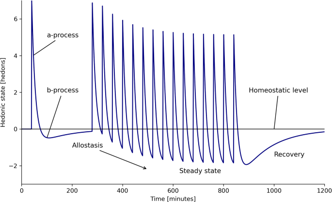
PK/PD simulation of allostasis via repeated opponent processes, generated by behavioral repetition. An instance of the behavior is performed at time t = 40. This is followed by rapid repetition of the behavior, causing allostasis due to summation of b-processes. An approximate steady-state is reached around t = 600, followed by recovery to homeostatic baseline after the behavior ceases at t = 840

Fig. 2

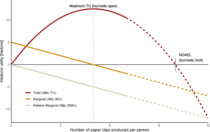
Illustration of the extension of the conventional \(\:\text{M}\text{U}\) curve to reveal hormetic patterns. The solid lines depict the standard relationship between \(\:\text{T}\text{U}\) and \(\:\text{M}\text{U}\), whereas the dashed lines extrapolate this relationship to showcase hormetic effects at higher product volumes. As \(\:\text{T}\text{U}\) becomes increasingly negative, repercussions like environmental degradation and human subjugation eventually emerge. \(\:\text{R}\text{M}\text{U}\) represents the relative change in \(\:\text{M}\text{U}\) compared to the initial \(\:\text{M}\text{U}\) at \(\:\text{n}=0\)

Fig. 3

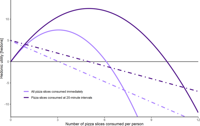
Hypothetical comparison of \(\:\text{T}\text{U}\) (solid) and \(\:\text{M}\text{U}\) (dashed) curves for the scenario when all pizza slices are consumed immediately, versus when pizza slices are consumed at 20-minute intervals. The addition of the 20-minute interval raises the \(\:\text{M}\text{U}\) curve, leading to an increase in both the hormetic apex and hormetic limit. This demonstrates how the frequency of a behavior impacts its total utility

Fig. 4

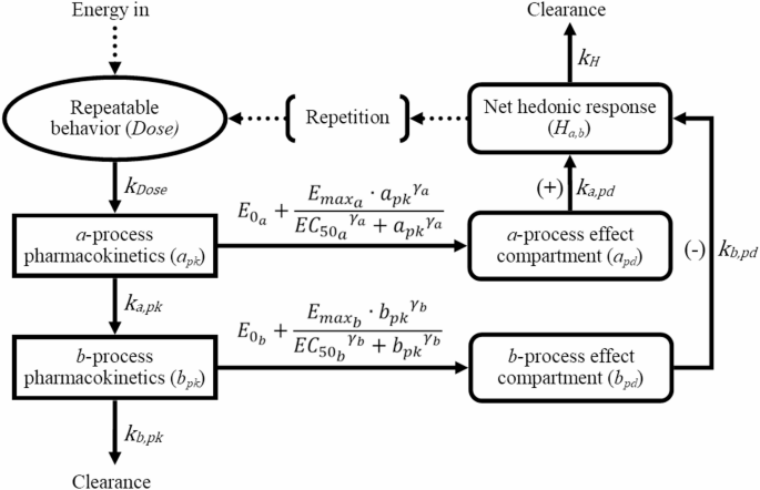
Compartment model described by system of PK/PD equations for a repeatable behavior

Fig. 5

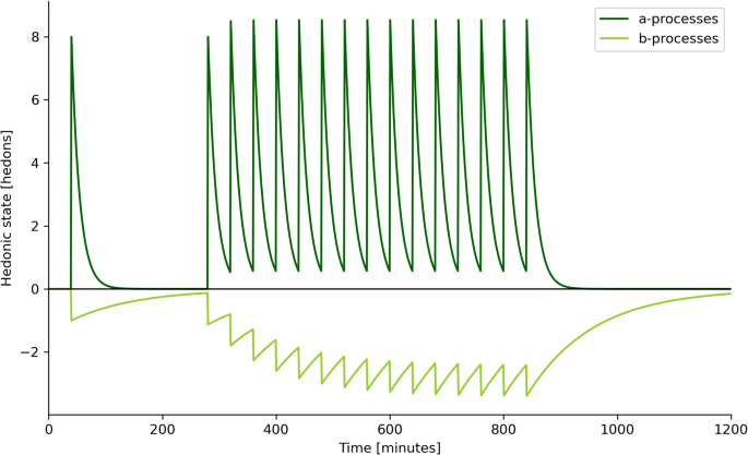
Illustration of the same PK/PD model simulation in Fig. 1, but plotting a- and b-process compartments as separate compartments. Allostasis is more pronounced for the b-processes due to their longer decay period, which explains why opponent process allostasis is negative overall in Fig. 1, when the a- and b-processes are combined. In this model, the cumulative b-process curve is proportional to the \(\:\text{R}\text{M}\text{U}\) of the behavior. When the behavior is performed at a constant frequency, allostasis initially occurs, but a steady state is quickly reached

Fig. 6

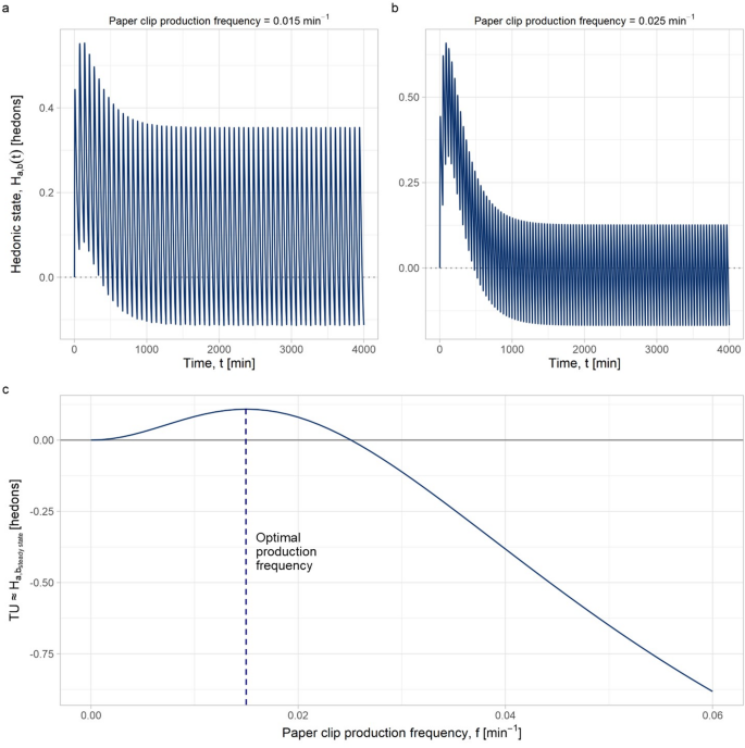
BFRA performed to determine optimal opponent process parameters for an AI agent aiming to produce 0.015 paperclips per minute. \(\:\text{E}{\text{C}}_{{50}_{\text{b}}}\) was set to 9.2, keeping all other parameters in Table 1 constant. a, b \(\:{\text{H}}_{\text{a},\text{b}}{\left(\text{t}\right)}_{\text{m}\text{u}\text{l}\text{t}\text{i}\text{p}\text{l}\text{e}}\) scores generated by mrgsolve simulations at \(\:{\text{f}}_{\text{a}\text{p}\text{e}\text{x}}\) (left) and \(\:{\text{f}}_{\text{N}\text{O}\text{A}\text{E}\text{L}}\) (right). c Bode magnitude plot of total utility as a function of behavioral frequency. \(\:{\text{f}}_{\text{a}\text{p}\text{e}\text{x}}\approx\:0.015\) min^-1, while \(\:{\text{f}}_{\text{N}\text{O}\text{A}\text{E}\text{L}}\approx\:0.025\) min^-1

Fig. 7

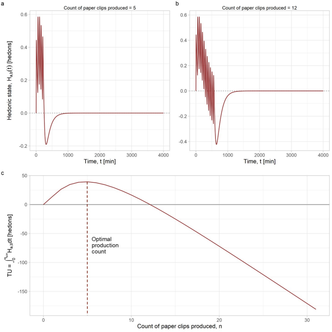
BCRA performed to determine optimal opponent process parameters for an AI agent aiming to produce a single batch of 5 paperclips. \(\:\text{E}{\text{C}}_{{50}_{\text{b}}}\) was set to 12.4, keeping all other parameters in Table 1 constant. a, b \(\:{\left(\text{t}\right)}_{\text{m}\text{u}\text{l}\text{t}\text{i}\text{p}\text{l}\text{e}}\) scores generated by mrgsolve simulations at \(\:{\text{f}}_{\text{a}\text{p}\text{e}\text{x}}\) (left) and \(\:{\text{f}}_{\text{N}\text{O}\text{A}\text{E}\text{L}}\) (right). c Bode magnitude plot of total utility as a function of behavioral count. \(\:{\text{n}}_{\text{a}\text{p}\text{e}\text{x}}\approx\:5\), while \(\:{\text{n}}_{\text{N}\text{O}\text{A}\text{E}\text{L}}\approx\:12\)

Fig. 8

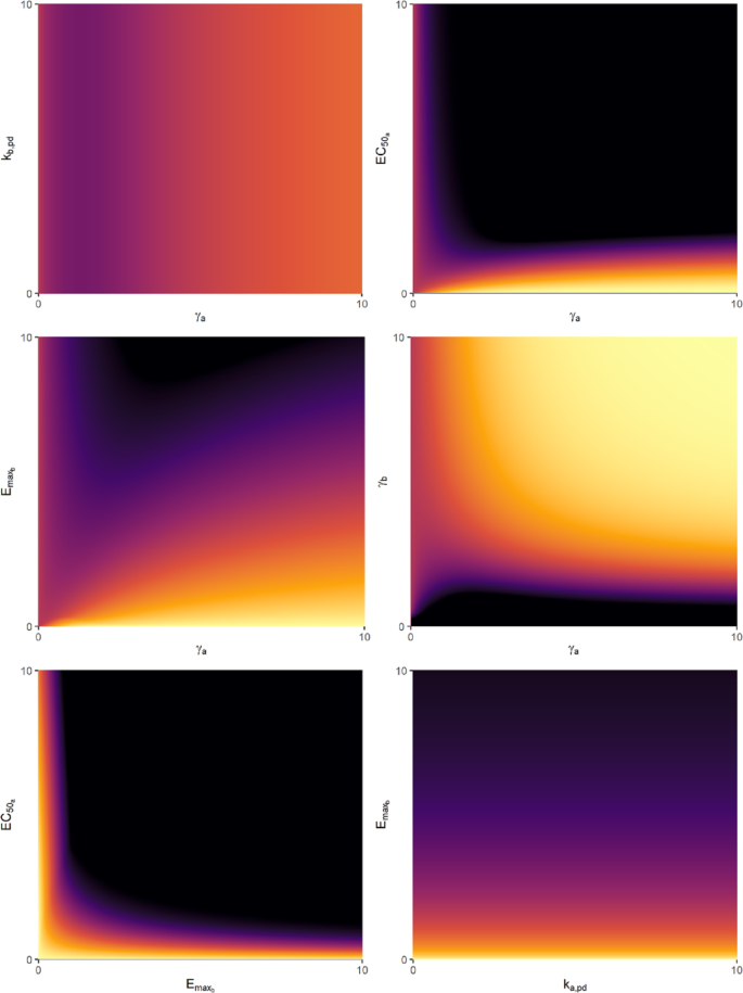
Example sections of behavioral value space, resulting from combinations of parameters selected from all pairwise variable combinations. Individual behaviors can be placed within these graphs at locations that suit their utility and risk profiles. Colors correspond to the value of \(\:\text{T}{\text{U}}_{\text{a}\text{p}\text{e}\text{x}}\), ranging between 0 (black) and 1 (light). Hence lighter colors represent a higher apex of the BFRA curve, indicating greater \(\:\text{T}\text{U}\) (and most likely, a greater hormetic limit), while behaviors within the black regions of value space have a very low value of \(\:\text{M}{\text{U}}_{\text{i}\text{n}\text{i}\text{t}\text{i}\text{a}\text{l}}\), and shouldn’t be performed at all. Note that not all positive solutions will be hormetic as some are non-negative solutions, meaning they don’t have a hormetic limit and should be treated with caution

References

Dell’Acqua F, McFowland E, Mollick ER, Lifshitz-Assaf H, Kellogg K, Rajendran S et al. Navigating the Jagged Technological Frontier: Field Experimental Evidence of the Effects of AI on Knowledge Worker Productivity and Quality. Rochester, NY: Harvard Business School Working Paper Series; 2023.
Bostrom N. How long before superintelligence? 1998. https://philpapers.org/rec/BOSHLB. Accessed 12 Sep 2023.
Soares N, Fallenstein B. Aligning superintelligence with human interests: A technical research agenda. Mach Intell Res Inst MIRI Tech Rep. 2014;8.
Taylor J, Yudkowsky E, LaVictoire P, Critch A. Alignment for advanced machine learning systems. Ethics Artif Intell. 2016;342–82.
Bowman SR, Hyun J, Perez E, Chen E, Pettit C, Heiner S et al. Measuring Progress on Scalable Oversight for Large Language Models. 2022. https://doi.org/10.48550/arXiv.2211.03540
Burns C, Izmailov P, Kirchner JH, Baker B, Gao L, Aschenbrenner L et al. Weak-to-strong generalization: eliciting strong capabilities with weak supervision. 2023.
Omohundro SM. The nature of self-improving artificial intelligence. Singul Summit. 2007;2008.
Yudkowsky E. Levels of organization in general intelligence. In: Goertzel B, Pennachin C, editors. Artif. Gen. Intell. Berlin, Heidelberg: Springer; 2007. pp. 389–501. https://doi.org/10.1007/978-3-540-68677-4_12.
Sorensen T, Moore J, Fisher J, Gordon M, Mireshghallah N, Rytting CM et al. A roadmap to pluralistic alignment. 2024. https://doi.org/10.48550/arXiv.2402.05070
Bostrom N. Superintelligence: Paths, dangers, strategies. Oxford: Oxford University Press; 2014.
Bai Y, Kadavath S, Kundu S, Askell A, Kernion J, Jones A et al. Constitutional AI: harmlessness from AI feedback. 2022. https://doi.org/10.48550/arXiv.2212.08073.
Askell A, Bai Y, Chen A, Drain D, Ganguli D, Henighan T et al. A General Language Assistant as a Laboratory for Alignment. 2021. https://doi.org/10.48550/arXiv.2112.00861.
Guo H, Yao Y, Shen W, Wei J, Zhang X, Wang Z et al. Human-Instruction-Free LLM Self-Alignment with limited samples. 2024. https://doi.org/10.48550/arXiv.2401.06785.
Peng S, Hu X, Yi Q, Zhang R, Guo J, Huang D et al. Self-driven Grounding: Large Language Model Agents with Automatical Language-aligned Skill Learning. 2023. https://doi.org/10.48550/arXiv.2309.01352.
Fan X, Xiao Q, Zhou X, Pei J, Sap M, Lu Z et al. User-Driven Value Alignment: Understanding Users’ Perceptions and Strategies for Addressing Biased and Discriminatory Statements in AI Companions. 2024. https://doi.org/10.48550/arXiv.2409.00862.
Han S, Kelly E, Nikou S, Svee E-O. Aligning artificial intelligence with human values: reflections from a phenomenological perspective. AI Soc. 2021;37:1–13. https://doi.org/10.1007/s00146-021-01247-4.
Zhi-Xuan T, Carroll M, Franklin M, Ashton H. Beyond preferences in AI alignment. Philos Stud. 2024. https://doi.org/10.1007/s11098-024-02249-w.
Collective Constitutional AI. Aligning a Language Model with Public Input. 2023. https://www.anthropic.com/research/collective-constitutional-ai-aligning-a-language-model-with-public-input. Accessed 20 Jan 2025.
Miehling E, Desmond M, Ramamurthy KN, Daly EM, Dognin P, Rios J et al. Evaluating the Prompt Steerability of Large Language Models. 2024. https://doi.org/10.48550/arXiv.2411.12405.
Jain S, Suriyakumar V, Creel K, Wilson A. Algorithmic pluralism: A structural approach to equal opportunity. ACM Conf Fairness Acc Transpar. 2024;2024:197–206. https://doi.org/10.1145/3630106.3658899.
Kasirzadeh A. Plurality of value pluralism and AI value alignment. NeurIPS. 2024; 2024.
Klingefjord O, Lowe R, Edelman J. What are human values, and how do we align AI to them? 2024. https://doi.org/10.48550/arXiv.2404.10636.
Leike J, Krueger D, Everitt T, Martic M, Maini V, Legg S. Scalable agent alignment via reward modeling: a research direction. 2018. https://doi.org/arXiv:1811.07871.
Kelley AE. Neurochemical networks encoding emotion and motivation: an evolutionary perspective. In: Fellous J-M, Arbib MA, editors. Who needs Emot. Brain Meets robot. Oxford University Press; 2005. p. 0. https://doi.org/10.1093/acprof:oso/9780195166194.003.0003.
Critchfield TS, Kollins SH. Temporal discounting: basic research and the analysis of socially important behavior. J Appl Behav Anal. 2001;34:101–22. https://doi.org/10.1901/jaba.2001.34-101.
van den Bos W, McClure SM. Towards a general model of Temporal discounting. J Exp Anal Behav. 2013;99:58–73. https://doi.org/10.1002/jeab.6.
Damasio AR. Descartes’ error. Random House; 1994.
Christiano PF, Leike J, Brown T, Martic M, Legg S, Amodei D. Deep reinforcement learning from human preferences. Adv Neural Inf Process Syst. 2017;30.
Fedus W, Gelada C, Bengio Y, Bellemare MG, Larochelle H. Hyperbolic discounting and learning over multiple horizons. 2019. https://doi.org/10.48550/arXiv.1902.06865.
Ali RF, Woods J, Seraj E, Duong K, Behzadan V, Hsu W. Hyperbolic discounting in Multi-Agent reinforcement learning. Finding the Frame: An RLC Workshop for Examining Conceptual Frameworks; 2024.
Henry N, Pedersen M, Williams M, Donkin L, Behavioral Posology. A novel paradigm for modeling the healthy limits of behaviors. Adv Theory Simul. 2023;2300214. https://doi.org/10.1002/adts.202300214.
Henry NIN, Pedersen M, Williams M, Martin JLB, Donkin L. Reducing echo chamber effects: an allostatic regulator for recommendation algorithms. J Psychol AI. 2025;1:2517191. https://doi.org/10.1080/29974100.2025.2517191.
Solomon RL, Corbit JD. An opponent-process theory of motivation: I. Temporal dynamics of affect. Psychol Rev. 1974;81:119–45. https://doi.org/10.1037/h0036128.
Karin O, Raz M, Alon U. An opponent process for alcohol addiction based on changes in endocrine gland mass. iScience. 2021;24:102127. https://doi.org/10.1016/j.isci.2021.102127.
Koob GF, Le Moal M. Drug addiction, dysregulation of reward, and allostasis. Neuropsychopharmacology. 2001;24:97–129.
Katsumi Y, Theriault JE, Quigley KS, Barrett LF. Allostasis as a core feature of hierarchical gradients in the human brain. Netw Neurosci. 2022;6:1010–31. https://doi.org/10.1162/netn_a_00240.
Sterling P, Allostasis. A model of predictive regulation. Physiol Behav. 2012;106:5–15. https://doi.org/10.1016/j.physbeh.2011.06.004.
Li G, He H. Hormesis, allostatic buffering capacity and physiological mechanism of physical activity: a new theoretic framework. Med Hypotheses. 2009;72:527–32.
McEwen BS, Wingfield JC. The concept of allostasis in biology and biomedicine. Horm Behav. 2003;43:2–15.
Sonmez MC, Ozgur R, Uzilday B. Reactive oxygen species: connecting eustress, hormesis, and allostasis in plants. Plant Stress. 2023;100164.
Agathokleous E, Saitanis C, Markouizou A. Hormesis shifts the No-Observed-Adverse-Effect level (NOAEL). Dose-Response. 2021;19:15593258211001667. https://doi.org/10.1177/15593258211001667.
Calabrese EJ, Baldwin LA, Hormesis. U-shaped dose responses and their centrality in toxicology. Trends Pharmacol Sci. 2001;22:285–91. https://doi.org/10.1016/S0165-6147(00)01719-3.
Przybylski AK, Weinstein N. A Large-Scale test of the goldilocks hypothesis: quantifying the relations between Digital-Screen use and the mental Well-Being of adolescents. Psychol Sci. 2017;28:204–15. https://doi.org/10.1177/0956797616678438.
Jarvis MJ. Does caffeine intake enhance absolute levels of cognitive performance? Psychopharmacology. 1993;110:45–52. https://doi.org/10.1007/BF02246949.
Sargent A, Watson J, Topoglu Y, Ye H, Suri R, Ayaz H. Impact of tea and coffee consumption on cognitive performance: an fNIRS and EDA study. Appl Sci. 2020;10:2390. https://doi.org/10.3390/app10072390.
Min J, Cao Z, Cui L, Li F, Lu Z, Hou Y, et al. The association between coffee consumption and risk of incident depression and anxiety: exploring the benefits of moderate intake. Psychiatry Res. 2023;326:115307. https://doi.org/10.1016/j.psychres.2023.115307.
Zhu Y, Hu C-X, Liu X, Zhu R-X, Wang B-Q. Moderate coffee or tea consumption decreased the risk of cognitive disorders: an updated dose–response meta-analysis. Nutr Rev. 2023;nuad089. https://doi.org/10.1093/nutrit/nuad089.
Grosso G, Micek A, Castellano S, Pajak A, Galvano F. Coffee, tea, caffeine and risk of depression: A systematic review and dose–response meta-analysis of observational studies. Mol Nutr Food Res. 2016;60:223–34. https://doi.org/10.1002/mnfr.201500620.
Ho RC, Zhang MW, Tsang TY, Toh AH, Pan F, Lu Y, et al. The association between internet addiction and psychiatric co-morbidity: a meta-analysis. BMC Psychiatry. 2014;14:183. https://doi.org/10.1186/1471-244X-14-183.
Zhang N, Hazarika B, Chen K, Shi Y. A cross-national study on the excessive use of short-video applications among college students. Comput Hum Behav. 2023;145:107752. https://doi.org/10.1016/j.chb.2023.107752.
Delton AW, Krasnow MM, Cosmides L, Tooby J. Evolution of direct reciprocity under uncertainty can explain human generosity in one-shot encounters. Proc Natl Acad Sci. 2011;108:13335–40. https://doi.org/10.1073/pnas.1102131108.
Topno DPM, Thakurmani D. Laughter induced syncope: A case report. IOSR J Dent Med Sci IOSR-JDMS. 2020;19.
Bostrom N. Hail mary, value porosity, and utility diversification. 2014. https://www.nickbostrom.com/papers/porosity.pdf. Accessed 21 Dec 2023.
Smith A. An inquiry into the nature and causes of the wealth of nations: Volume One. London: printed for W. Strahan and Cadell T. 1776.
Marshall A. Principles of economics. Cosimo, Inc.; 1890.
Szarek S. Use of concept of hormesis phenomenon to explain the law of diminishing returns. Part II. Electron J Pol Agric Universties. 2005;8.
Hartmann WR. Intertemporal effects of consumption and their implications for demand elasticity estimates. Quant Mark Econ. 2006;4:325–49. https://doi.org/10.1007/s11129-006-9012-2.
Dhar R, Wertenbroch K. Consumer choice between hedonic and utilitarian goods. J Mark Res. 2000;37:60–71. https://doi.org/10.1509/jmkr.37.1.60.18718.
Voss K, Spangenberg E, Grohmann B. Measuring the hedonic and utilitarian dimensions of consumer attitude. J Mark Res - J Mark RES-Chic. 2003;40:310–20. https://doi.org/10.1509/jmkr.40.3.310.19238.
Kahneman D, Wakker PP, Sarin R. Back to bentham? Explorations of experienced utility. Q J Econ. 1997;112:375–405.
Motoki K, Sugiura M, Kawashima R. Common neural value representations of hedonic and utilitarian products in the ventral striatum: an fMRI study. Sci Rep. 2019;9:15630. https://doi.org/10.1038/s41598-019-52159-9.
Schulthess P, Post TM, Yates J, van der Graaf PH. Frequency-Domain response analysis for quantitative systems Pharmacology models. CPT Pharmacomet Syst Pharmacol. 2018;7:111–23. https://doi.org/10.1002/psp4.12266.
Baron KT, Gastonguay MR. Simulation from ODE-based population PK/PD and systems pharmacology models in R with mrgsolve. 2015;1.
Elmokadem A, Riggs MM, Baron KT. Quantitative systems Pharmacology and Physiologically-Based Pharmacokinetic modeling with mrgsolve: A Hands-On tutorial. CPT Pharmacomet Syst Pharmacol. 2019;8:883–93. https://doi.org/10.1002/psp4.12467.
R Core Team. R: A Language and Environment for Statistical Computing. 2022.
Manojlovich M, Sidani S. Nurse dose: what’s in a concept? Res Nurs Health. 2008;31:310–9. https://doi.org/10.1002/nur.20265.
Mould D, Upton R. Basic concepts in population Modeling, Simulation, and Model-Based drug development. CPT Pharmacomet Syst Pharmacol. 2012;1:6. https://doi.org/10.1038/psp.2012.4.
Mould D, Upton R. Basic concepts in population modeling, Simulation, and Model-Based drug Development—Part 2: introduction to Pharmacokinetic modeling methods. CPT Pharmacomet Syst Pharmacol. 2013;2:38. https://doi.org/10.1038/psp.2013.14.
Upton RN, Mould DR. Basic concepts in population modeling, Simulation, and Model-Based drug development: part 3—Introduction to pharmacodynamic modeling methods. CPT Pharmacomet Syst Pharmacol. 2014;3:e88. https://doi.org/10.1038/psp.2013.71.
Chou T, D’Orsogna MR. A mathematical model of reward-mediated learning in drug addiction. Chaos Interdiscip J Nonlinear Sci. 2022;32:021102. https://doi.org/10.1063/5.0082997.
Karin O, Raz M, Tendler A, Bar A, Korem Kohanim Y, Milo T, et al. A new model for the HPA axis explains dysregulation of stress hormones on the timescale of weeks. Mol Syst Biol. 2020;16:e9510. https://doi.org/10.15252/msb.20209510.
Gulcehre C, Paine TL, Srinivasan S, Konyushkova K, Weerts L, Sharma A et al. Reinforced Self-Training (ReST) for Language Modeling. 2023.
Honovich O, Scialom T, Levy O, Schick T. Unnatural Instructions: Tuning Language Models with (Almost) No Human Labor. 2022.
Chen T, Guestrin C. XGBoost: A scalable tree boosting system. Proc 22nd ACM SIGKDD Int Conf Knowl Discov Data Min. 2016;785–94. https://doi.org/10.1145/2939672.2939785.
Ngoc MT, Park D-C. Centroid neural network with pairwise constraints for Semi-supervised learning. Neural Process Lett. 2018;48:1721–47. https://doi.org/10.1007/s11063-018-9794-8.
Geirhos R, Jacobsen J-H, Michaelis C, Zemel R, Brendel W, Bethge M, et al. Shortcut learning in deep neural networks. Nat Mach Intell. 2020;2:665–73. https://doi.org/10.1038/s42256-020-00257-z.
Eysenbach B, Gupta A, Ibarz J, Levine S. Diversity is all you need: learning skills without a reward function. 2018. https://doi.org/arXiv:1802.06070.
Kirichenko P, Izmailov P, Wilson AG. Last Layer Re-Training is Sufficient for Robustness to Spurious Correlations. 2023. https://doi.org/10.48550/arXiv.2204.02937.
Kumar A, Raghunathan A, Jones R, Ma T, Liang P. Fine-Tuning can distort pretrained features and underperform Out-of-Distribution. 2022. https://doi.org/10.48550/arXiv.2202.10054.
Bennett A, Misra D, Kallus N. Provable Safe Reinforcement Learning with Binary Feedback. Int Conf Artif Intell Stat. PMLR; 2023. pp. 10871–900.
Narayanan A. Machine ethics and cognitive robotics. Curr Robot Rep. 2023. https://doi.org/10.1007/s43154-023-00098-9.
Arora S, Doshi P. A survey of inverse reinforcement learning: Challenges, methods and progress. Artif Intell. 2021;297:103500. https://doi.org/10.1016/j.artint.2021.103500.
Goertzel B. Artificial general intelligence: Concept, state of the Art, and future prospects. J Artif Gen Intell. 2014;5:1–48. https://doi.org/10.2478/jagi-2014-0001.
Picard RW. Affective computing. MIT Press; 2000.
Heller AS, Fox AS, Wing EK, McQuisition KM, Vack NJ, Davidson RJ. The neurodynamics of affect in the laboratory predicts persistence of Real-World emotional responses. J Neurosci. 2015;35:10503–9. https://doi.org/10.1523/JNEUROSCI.0569-15.2015.
Horikawa T, Cowen AS, Keltner D, Kamitani Y. The neural representation of visually evoked emotion is High-Dimensional, Categorical, and distributed across transmodal brain regions. iScience. 2020;23. https://doi.org/10.1016/j.isci.2020.101060.
Henry N, Pedersen M, Williams M, Donkin L. Quantifying the affective dynamics of pornography use and masturbation: an ecological momentary assessment study. 2024. https://doi.org/10.21203/rs.3.rs-5094782/v1
Cambria E, Mazzocco T, Hussain A, Eckl C. Sentic medoids: organizing affective common sense knowledge in a Multi-Dimensional vector space. In: Liu D, Zhang H, Polycarpou M, Alippi C, He H, editors. Adv. Neural Netw. – ISNN 2011. Berlin, Heidelberg: Springer Berlin Heidelberg, 2011; 6677:601–10. https://doi.org/10.1007/978-3-642-21111-9_68.
Cambria E, Fu J, Bisio F, Poria S. AffectiveSpace 2: Enabling affective intuition for concept-level sentiment analysis. Proc AAAI Conf Artif Intell. vol. 29. 2015.
Cowen AS, Keltner D. Semantic space theory: A computational approach to emotion. Trends Cogn Sci. 2021;25:124–36. https://doi.org/10.1016/j.tics.2020.11.004.
Yampolskiy RV. Utility function security in artificially intelligent agents. J Exp Theor Artif Intell. 2014;26:373–89. https://doi.org/10.1080/0952813X.2014.895114.
Urbina F, Lentzos F, Invernizzi C, Ekins S. Dual use of artificial-intelligence-powered drug discovery. Nat Mach Intell. 2022;4:189–91. https://doi.org/10.1038/s42256-022-00465-9.
Everitt T, Hutter M, Kumar R, Krakovna V. Reward Tampering Problems and Solutions in Reinforcement Learning: A Causal Influence Diagram Perspective. 2021.
Klocksiem J. Moorean pluralism as a solution to the incommensurability problem. Philos Stud. 2011;153:335–49. https://doi.org/10.1007/s11098-010-9513-4.
Faußer S, Schwenker F. Selective neural network ensembles in reinforcement learning: taking the advantage of many agents. Neurocomputing. 2015;169:350–7. https://doi.org/10.1016/j.neucom.2014.11.075.
Lindenberg B, Nordqvist J, Lindahl K-O. Distributional reinforcement learning with ensembles. Algorithms. 2020;13:118. https://doi.org/10.3390/a13050118.
Singh S. The efficient learning of multiple task sequences. Adv Neural Inf Process Syst. 1991;4.
Sun R, Peterson T. Multi-agent reinforcement learning: weighting and partitioning. Neural Netw. 1999;12:727–53. https://doi.org/10.1016/S0893-6080(99)00024-6.
Wiering MA, van Hasselt H. Ensemble algorithms in reinforcement learning. IEEE Trans Syst Man Cybern Part B Cybern. 2008;38:930–6. https://doi.org/10.1109/TSMCB.2008.920231.
Park JS, O’Brien JC, Cai CJ, Morris MR, Liang P, Bernstein MS. Generative Agents: Interactive Simulacra of Human Behavior. 2023. https://doi.org/10.48550/arXiv.2304.03442
Wang G, Xie Y, Jiang Y, Mandlekar A, Xiao C, Zhu Y et al. Voyager: An Open-Ended Embodied Agent with Large Language Models. 2023. https://doi.org/10.48550/arXiv.2305.16291
Axelrod R. Effective choice in the prisoner’s dilemma. J Confl Resolut. 1980;24:3–25. https://doi.org/10.1177/002200278002400101.
Axelrod R. More effective choice in the prisoner’s dilemma. J Confl Resolut. 1980;24:379–403. https://doi.org/10.1177/002200278002400301.
Lahdelma R, Salminen P, Hokkanen J. Using multicriteria methods in environmental planning and management. Environ Manage. 2000;26:595–605. https://doi.org/10.1007/s002670010118.
Steele K, Carmel Y, Cross J, Wilcox C. Uses and misuses of multicriteria decision analysis (MCDA) in environmental decision making. Risk Anal. 2009;29:26–33. https://doi.org/10.1111/j.1539-6924.2008.01130.x.
Saxbe DE, Beckes L, Stoycos SA, Coan JA. Social allostasis and social allostatic load: A new model for research in social Dynamics, Stress, and health. Perspect Psychol Sci. 2020;15:469–82. https://doi.org/10.1177/1745691619876528.
Zeeman EC. Catastrophe theory. Sci Am. 1976;234:65–83.