Abyssal seafloor as a key driver of ocean trace-metal biogeochemical cycles

Many trace elements are essential nutrients for marine life and have a key role in the carbon cycle¹. They are also indispensable tools for investigating the evolution of the ocean and climate systems in Earth history¹. Studying their marine cycles is vital for safeguarding marine ecosystems and understanding past and current climate change. Historically, interpretations of trace-element cycles have followed a top-down ‘nutrient-type’ model²¹. Reversible scavenging, a leading mechanism, proposes that the decreasing concentration of scavenging particles with depth releases surface-sourced elements^3,4,5. This mechanism was first applied to thorium (Th) isotopes²; however, they have radioactive decay sources in the water column to support their concentration increase with depth. For other elements, ocean biogeochemical models (OBMs) generally assume that remineralization of biogenic particles provides the internal source^3,4,5. Such models often ignore manganese (Mn) and iron (Fe) oxides, despite the fact that they are established scavengers^11,22, as evidenced in the latest GEOTRACES studies^23,24,25,26.

Recent discoveries of widespread sedimentary imprints on the distributions of many trace elements and isotopes (TEIs), such as Fe (refs. ^27,28), neodymium (Nd)^6,8,9, beryllium (Be)¹⁰, lead (Pb)²⁹, nickel (Ni)³⁰, copper (Cu)³¹, chromium (Cr)³² and their isotopes, are discordant with the top-down view. An alternative boundary-exchange view argues that particle-dissolved exchange at ocean boundaries drives trace-element cycles^6,7,12. A bottom-up diagenetic benthic flux is a favoured candidate to explain boundary exchange, supported by observational^{10,19,20,28,32,33} and modelling evidence^13,15,31,34. But it remains unclear what processes facilitate sedimentary influences on the water column and how the benthic flux is linked to particle scavenging.

Critically, the top-down and bottom-up models can imply completely different behaviours of TEIs as tracers of ocean processes. For example, seawater radiogenic Nd isotope composition (ε_Nd) has been used as a conservative water-mass mixing tracer assuming that external sources of Nd exist only at the surface³⁵; however, recent arguments for a strong benthic control propose ε_Nd as a non-conservative tracer of abyssal circulation rate^9,33,36, or in extreme cases, a proxy of local sediment provenance^8,9. Understanding the relative importance of top-down versus bottom-up processes is thus essential.

So far, studies of particle scavenging and boundary exchange are heavily biased towards the upper ocean, where biogenic particles are most abundant, and continental margins, where reducing sediment environments often dominate. However, emerging evidence based on seawater Fe (ref. ³⁷) and Nd (ref. ⁹) isotopes and porewater geochemistry^20,33 suggests that the oxic abyssal seafloor, long overlooked, can host important biogeochemical transformations. Moreover, recent ocean-mixing studies have revealed that the abyssal ocean generates surprisingly strong turbulence through interaction of internal tides with seafloor topography, creating bottom-intensified diapycnal mixing that sustains the overturning circulation^16,17. Considering the areal extent of this benthic mixing, any geochemical exchange at the abyssal seafloor should be quantitatively important.

Here we report water-column, sediment and porewater data from the abyssal central Pacific. We use these data to constrain a model that constitutes an integrated framework for describing marine trace-element cycling from the water column to abyssal sediment that stresses the importance of benthic impacts. We use rare earth elements (REE; including Nd) and Nd isotopes to constrain the model, exploiting their proven utility in studying particle scavenging, ocean mixing and boundary exchange^6,7,11,35. Neodymium has the advantage that its residence time is relatively short (about 400–500 yr)⁹, such that circulation does not mask the impacts of particle scavenging and benthic flux; but long enough to be a tracer of basinal to global, rather than local, processes. We use these tracers to develop a broader concept: the interplay between particle scavenging and benthic processing is relevant to many trace elements. We focus on the abyssal Pacific, a quarter of Earth’s surface area, whose weak overturning allows the impact of biogeochemical cycling to manifest most clearly.

Marine particles are categorized into biogenic, lithogenic and authigenic types^22,25. For example, biogenic particles include soft tissues and mineral shells (for example, carbonate and opal), each with different processes controlling the nature and length scales of remineralization^3,13. Authigenic phases, precipitating from seawater or pore water, are best exemplified by Mn and Fe (oxyhydr)oxides, as macroscopic structures (for example, nodules) or microscopic coatings on other particles²². Marine particles in nature are a mix of all three types, and thus isolating them into their respective fractions is needed to better understand scavenging dynamics.

We quantitatively attributed the association of scavenged REE using partition coefficients^23,24,25,26 (K_d) estimated with the global GEOTRACES data³⁸ (see ‘Particle scavenging’ in Methods). The result shows that Nd has the greatest affinity for Mn oxide (log₁₀K_d, 8.76 median value, 8.72–8.79 interquartile range), followed by Fe oxide (7.26, 7.21–7.37), both being much greater than particulate organic matter (POM; 5.93, 5.86–6.01), whereas carbonate, opal and lithogenic particles are probably insignificant especially in the deep ocean, consistent with previous regional studies^23,26. This affinity pattern is similar to that of Th, protactinium (Pa), polonium (Po) and Pb (refs. ^24,39), demonstrating the potency of Mn oxide in scavenging a wide range of TEIs. Beneath the surface, Mn oxide makes up less than 1% of the particle mass but accounts for approximately 50–90% of scavenged Nd in the Pacific (Fig. 1).

Fig. 1: Particle scavenging in the Pacific.

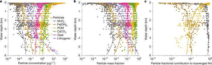
a,b, Particle concentration (a) and mass fraction (b) from the Pacific GEOTRACES data^25,38. c, Estimated particulate contribution to scavenged Nd using data-constrained K_d; carbonate, opal and lithogenic particles are not significant scavengers and are not shown (see ‘Particle scavenging’ in Methods). Despite being the least abundant scavenging phase, authigenic Mn oxide makes the predominant contribution to Nd scavenging. Lines in the plots are either power-law (biogenic particles) or locally estimated scatterplot smoothing (LOESS) (other particle types) trends with depth.

Our abyssal (below 5,000 m water depth) sediment data agree with this water-column result. From the biogenic-rich Station 4 at the border of the productive equatorial upwelling zone, to the red-clay-site Station 3 underlying the oligotrophic gyre (Fig. 2a and ‘Pacific cruise’ in Methods), sediment REE are dominantly found in authigenic fractions (see ‘Abyssal Pacific sediment’ in Methods), including 76 ± 9% Nd (1σ). The consistency of authigenic enrichment across our sites, despite an approximately fivefold change of sinking biogenic particle flux⁴⁰, shows that biogenic particles are negligible carriers of REE. Authigenic sediments also account for 89 ± 6% of Mn but for only 26 ± 16% of Fe. The authigenic Mn/Fe ratio (0.3–1.3, 95% range) is much higher than for the upper continental crust⁴¹ (0.02), suggesting the prevalence of Mn oxide. The geochemical compositions of water-column authigenic particles and abyssal authigenic sediments are similar, both resembling those of oxide-rich phases (Extended Data Fig. 1 and ‘REE carriers’ in Methods). Such similarity points to the highly consistent geochemical nature of oxides across a wide range of environmental conditions.

Fig. 2: Pacific sites and biogeochemistry.

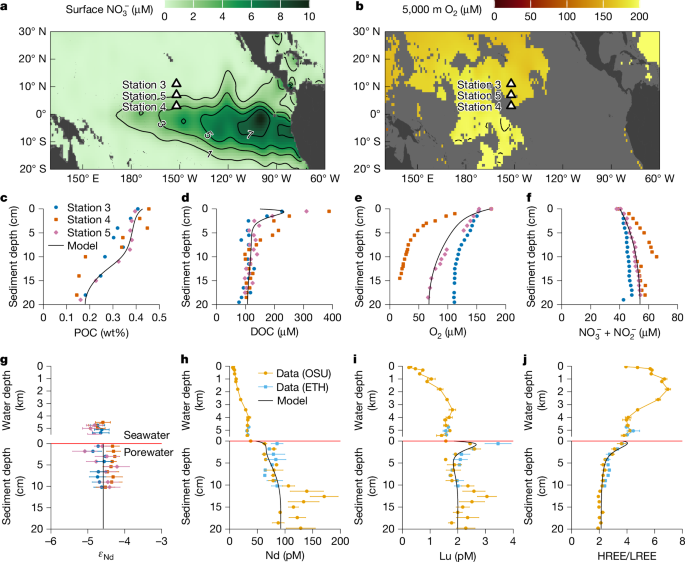
a, Surface-ocean nitrate concentrations⁵⁶. b, Oxygen concentration at 5,000 m water depth⁵⁶. c–f, Concentrations of sediment particulate organic carbon (POC; c), porewater dissolved organic carbon (DOC; d), oxygen (O₂; e) and nitrate + nitrite (NO₃⁻ + NO₂⁻; f). g–j, Seawater and porewater profiles of ε_Nd (with 2σ error bars; g), Nd (h) and Lu (i) concentrations, and HREE/LREE ratios (that is, [Tm + Yb + Lu]/[La + Pr + Nd] using shale-normalized concentrations; j). In c–g, data are measured in the same lab and we plot the three sites separately (see ‘Pacific cruise’ in Methods). In h–j, data are measured at both Oregon State University (OSU) and ETH Zurich (ETH) and we show the mean values of the three sites and the standard errors of the mean values. The black lines in c–j are modelled values. See ‘Diagenetic model’ in Methods and Extended Data Figs. 2 and 3 for detailed model description and results.

We further found an agreement between the particle rain and sediment burial rates of REE, establishing the consistency of water-column-to-sediment mass transfer. Combining published particle concentration data with sediment-trap-based mass flux data in the study region (see ‘Water-column and sediment mass fluxes’ in Methods), we estimate that the rain rates of authigenic and total particulate Nd are 55 ± 24 (1σ) pmol cm⁻² yr⁻¹ and 68 ± 27 pmol cm⁻² yr⁻¹, respectively, agreeing with the estimated burial rates of 53 ± 17 pmol cm⁻² yr⁻¹ and 62 ± 20 pmol cm⁻² yr⁻¹, respectively.

Integrating these independent lines of evidence, we conclude that Mn oxide is the dominant host of water-column and surface-sediment REE. Essentially, abyssal sediments accumulate oxide-scavenged water-column trace elements, with less lithogenic and small biogenic contributions. Post-depositional processes are not needed to explain metal enrichment in abyssal sediments: they probably only act to redistribute REE among the solid phases, for example, conversion from disordered to stable oxides⁴² and transfer from oxides to phosphates¹⁵, with limited impact on the sediment authigenic budget (see ‘REE carriers’ in Methods).

Despite the efficient scavenging by settling particles, abyssal pore water is enriched in REE over bottom seawater, implying a diffusive flux to the ocean (Fig. 2). We use reactive-transport modelling to illustrate how oxic diagenesis explains the observed benthic fluxes (see ‘Diagenetic model’ in Methods).

The apparent oxide K_d decreases from water column to sediment because POM remineralization lowers the pH and increases the organic ligand concentration in pore water (Extended Data Figs. 2 and 3). This change leads to net desorption of oxide-bound metals, despite the high absolute value of K_d. POM-bound metals are also released, representing an amount that is small in the particulate flux but substantial for the porewater budget (Extended Data Figs. 2 and 3). In comparison, on continental margins, porewater pH is strongly buffered by alkalinity released during diagenesis, and kinetic reduction of oxides is the dominant source of benthic flux whereas equilibrium sorption is negligible¹⁵.

Our diagenetic model can reproduce the porewater-profile-based measurements of benthic flux (2.9 ± 0.5 pmol cm⁻² yr⁻¹ for Nd; ‘Benthic fluxes’ in Methods), which is smaller than the sinking particle flux, suggesting relatively low recycling efficiency (approximately 5%). The model also reproduces the porewater REE pattern (Extended Data Fig. 3): oxides and POM release a light REE (LREE)-enriched source to pore water, whereas preferential formation of organic complexes creates heavy REE (HREE) concentration peaks close to the interface (Fig. 2).

Given the strong affinity of REE with oxides and the increase of oxide concentration with water depth (Fig. 1), we argue that scavenging constitutes a net removal from the water column. We tested this idea by creating a three-dimensional (3D) model of the Nd cycle using the transport matrix method^3,4,34 (see ‘Water-column model’ in Methods). We use the ocean circulation inverse model⁴³ with increased vertical resolution and state-of-the-art parameterization of bottom-intensified mixing¹⁶ (OCIM2-48L, 48 layers, 2° resolution). This model produces an improved representation of the abyssal Pacific circulation strongly shaped by seafloor topography^17,43, allowing for a robust evaluation of the potential bottom-up control of the marine Nd cycle.

Supplying only river and dust fluxes to the model, we reproduce the classic behaviour of metals in reversible scavenging OBMs^3,4,5,13: the dissolved element concentration increases with water depth as biogenic particles shuttle surface sources downwards (Fig. 3a and Extended Data Figs. 4 and 5). Here we use POM as the only biogenic scavenger, suggested by our analysis of the GEOTRACES data. The model can fit the Nd concentration profile in the upper water column only at the expense of underestimating the deeper Nd concentrations, making the profile more nutrient-like than the nearly linear observations. This OBM disparity issue is often overcome in the literature by specifying carbonate and opal as scavengers of trace elements^3,13, taking advantage of their longer remineralization length scales. We can reproduce similar results by allowing the K_d of these biogenic particles to be free tuning parameters (Extended Data Fig. 4), but our analysis of GEOTRACES data (Fig. 1) shows that such model exercises are not consistent with observations.

Fig. 3: Seafloor imprint on water-column Nd concentration in the Pacific.

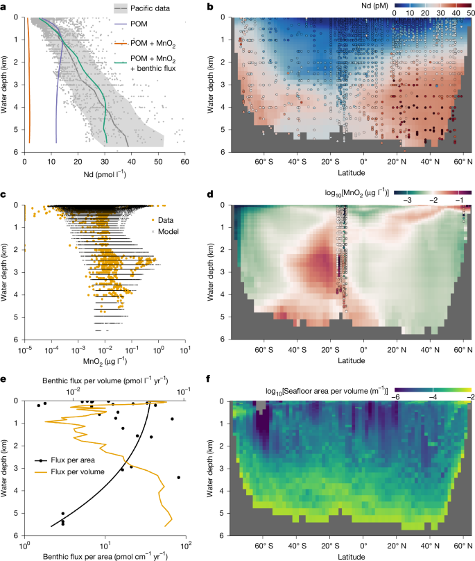
a,b, Results of model experiments (see ‘Water-column model’ in Methods), including scavenging with: (1) POM only; (2) with added MnO₂ scavenging; and (3) with added benthic flux. a, Modelled horizontally averaged concentrations of all three experiments. b, Modelled zonal mean concentrations for experiment (3) (see Extended Data Fig. 4 for scavenging by other biogenic particles, and Extended Data Fig. 5 for results of experiments (1) and (2)). Compiled Pacific seawater data are indicated by grey dots in a and colour-coded dots in b (see ‘Nd data compilation’ in Methods). The mean values and 1σ range of the data are shown by the grey line and shading, respectively, in a. c,d, Estimated particulate MnO₂ concentrations (see ‘Water-column model’ in Methods; also see Extended Data Fig. 6). The GEOTRACES data^25,38 are compared with neural-network-derived results on the model grids in c, and the zonally averaged concentrations (background colour) are shown in d together with GEOTRACES data (coloured dots). e,f, Benthic flux and the geometry of the ocean basin⁵⁷, showing the depth distributions of benthic flux per unit area and unit volume (horizontal average; e) and seafloor-area-to-volume ratio (zonal average; f). In e, the black dots are porewater-based estimates of per unit area flux (see ‘Water-column model’ in Methods), the black line is its depth profile used in the model and the yellow line is the corresponding per unit volume flux. This flux profile is not made to best-fit the existing data, which is highly scarce, but to demonstrate that given reasonable estimates of benthic flux within the constraint of the data, we can explain the depth profiles of seawater Nd. In f, the area-to-volume ratio is computed using subgrid bathymetry based on ETOPO 2022⁵⁷ (also see Extended Data Fig. 7).

To implement oxide scavenging, we generate a 3D Mn oxide concentration field by training an artificial neural network using GEOTRACES data^25,38 (Extended Data Fig. 6 and ‘Water-column model’ in Methods). Once we add Mn oxide to the model, scavenging becomes a net sink of Nd throughout the water column (Fig. 3a–d and Extended Data Figs. 4 and 5). Although scavenging is implemented as a reversible mechanism, the net result appears as an irreversible process. This result illustrates that, for metals with an affinity for Mn oxide much greater than for biogenic particles, their increasing concentrations with water depth requires either an internal (for example, Th) or a boundary source (for example, REE).

We propose that benthic fluxes, originating mostly from the abyssal seafloor, explain the water-column REE concentration increase for two reasons.

First, the shape of ocean basins is such that the abyssal ocean has the most seafloor area but only a fraction of the ocean volume, resulting in an exponential increase of the area-to-volume ratio with water depth (Fig. 3e,f and Extended Data Fig. 7a,b). Although the continental margins have much higher benthic flux per unit area⁴⁴, the abyssal seafloor dominates the total sedimentary flux because of its areal predominance (Fig. 3e). Consequently, in the abyssal ocean, even a small benthic flux per unit area has a large impact on metal concentration per unit volume.

Second, diapycnal diffusivity increases exponentially from about 10⁻⁵ m² s⁻¹ in the upper ocean to about 10⁻³ m² s⁻¹ in the abyss because of the turbulence generated by internal tides impinging on seafloor topography¹⁶ (Extended Data Fig. 7c and ‘Bottom-intensified mixing’ in Methods). Accordingly, the diffusion length of Nd increases with depth from about 1 km to about 5 km (Extended Data Fig. 7d), implying a large vertical impact of abyssal benthic sources.

Adding a benthic flux to our model successfully simulates the first-order feature that Nd concentration increases nearly linearly with depth in the Pacific (Fig. 3a,b, Extended Data Fig. 5 and ‘Water-column model’ in Methods). Superimposed on this large-scale distribution, our model also captures the spatial heterogeneity owing to localized factors such as hydrothermal plumes and nepheloid layers near the East Pacific Rise (Fig. 3 and Extended Data Fig. 6). The model underestimates abyssal Pacific Nd concentrations near 40° N, where a previous study used radium (Ra) isotopes to infer anomalously high benthic flux and/or sluggish mixing⁴⁵. Such regional features are not included in our large-scale model. Overall, our model clearly illustrates how the dynamic interplay between scavenging and benthic source controls the water-column metal distribution, seen clearly in the Nd cycle owing to its moderate residence time (466 years in this model).

The results above demonstrate the potentially dominant control of boundary exchange on water-column concentration profiles. Here we further show that the abyssal benthic flux is capable of transforming water-column isotope distributions on large scales. In the classic top-down-only view^3,35, water-mass endmembers acquire their ε_Nd signatures at the surface ocean, and in the interior seawater, the ε_Nd distribution reflects conservative mixing of these endmembers. This view is inconsistent with the observation that abyssal Pacific ε_Nd is non-conservative, as shown by the strong correlation of ε_Nd with water-mass age^9,36 (Fig. 4a). There is no deep-water formation in the North Pacific, and the predominant deep-water source is from the well-mixed Southern Ocean, which has ε_Nd of about −9 ε (Extended Data Fig. 8 and ‘Nd data compilation’ in Methods). As deep water traverses northwards, ε_Nd becomes increasingly radiogenic (more positive ε_Nd values), reaching >−4 ε in the North Pacific (Fig. 4a). Reversible scavenging has been argued to bring radiogenic surface water signatures to the deep ocean³, but OBMs have struggled to simulate the observed ε_Nd of Pacific Deep Water^13,46.

Fig. 4: Seafloor imprint on water-column ε_Nd in the Pacific.

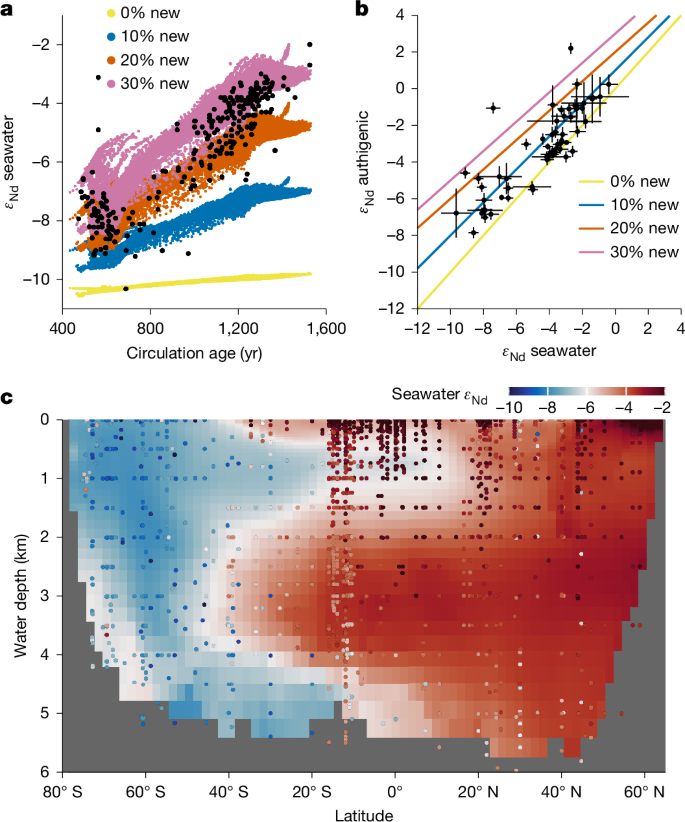
a, Abyssal (>3,000 m) ocean ε_Nd is altered towards more radiogenic (that is, positive) values with increasing water-mass age, because of prolonged exposure to a new benthic flux driven by weathering of sedimentary volcanic silicates. The black dots indicate seawater data and the coloured dots indicate the model grid. The colour refers to the model experiment, in which the new source accounts for 0% to 30% of the total benthic flux (see ‘Water-column model’ in Methods). In these experiments, the new source is added to all seafloor areas in the Pacific. Extended Data Fig. 10 shows experiments of adding the new source to various subregions of the seafloor. b, Relationship between the ε_Nd of authigenic sediment and overlying seawater, indicating that new sources are needed to explain the authigenic data. Paired observations are binned into ocean boxes and indicated by black dots with standard deviations (see ‘Nd data compilation’ in Methods and Extended Data Fig. 8); the coloured lines indicate mixing between seawater and 0% to 30% of new benthic source. c, Modelled zonally averaged seawater ε_Nd in the experiment where we add 30% new source to all Pacific seafloor areas (see Extended Data Fig. 9 for experiments with approximately 0–20% new source). Compiled Pacific data are indicated by coloured dots.

We adopt concepts from nutrient cycling, and partition the benthic flux into a recycled component owing to the regeneration of water-column scavenged Nd, and a newly introduced (‘new’) component arising from in situ marine silicate weathering^{6,8,12,14,15,33,47}. Surface water ε_Nd in the study region is radiogenic (about −3 ε to 0 ε; Extended Data Fig. 8), whereas porewater and bottom-water ε_Nd are similar at about −4.5 ε (Fig. 2). This similarity indicates that the abyssal benthic flux in the study region is mainly recycled, and regenerated Nd is primarily scavenged from the deep ocean. Following the water-column cycling model above, such a recycled flux readily explains the non-conservative increase of Nd concentration, but it has little power to alter abyssal ε_Nd.

In contrast, a new benthic flux derived from weathering of volcanic silicates (ε_Nd ≈ +10) sourced from the Pacific Ring of Fire would explain the non-conservativity of ε_Nd (refs. ^6,8,15,47). We tested this idea by incorporating Nd isotopes in the water-column model (see ‘Water-column model’ in Methods). Our experiments show that, without a new source, reversible scavenging has limited power to explain the radiogenic nature of Pacific Deep Water, and the abyssal Pacific simply inherits the ε_Nd of its Southern Ocean source waters (Fig. 4a and Extended Data Fig. 9). In contrast, with a new component constituting 10% to 30% of the total benthic flux added to all seafloor areas in the Pacific, prolonged exposure to this flux owing to weak meridional circulation transforms the abyssal Pacific ε_Nd towards observed radiogenic values (Fig. 4a,c and Extended Data Fig. 9). Sediment studies are consistent with this partition of benthic flux. In the Northeast Pacific, the only other location with porewater ε_Nd data, benthic fluxes are more radiogenic than bottom water, allowing for up to 20% new component in the larger benthic fluxes found there³³. Authigenic sediments in the Pacific are also consistently more radiogenic than bottom water⁹; if these authigenic data mirror porewater ε_Nd (refs. ^33,47), they too are consistent with a 10% to 30% new benthic flux component (Fig. 4b). In comparison, our model results show that even greater proportions of new benthic flux is needed to explain the highly radiogenic ε_Nd of intermediate waters (Fig. 4c), for example in the equatorial western Pacific where intense boundary exchange with basaltic islands was discovered⁶.

Model sensitivity experiments further show that abyssal seawater ε_Nd cannot be explained if boundary exchange is restricted to the margins (see ‘Water-column model’ in Methods). Limiting the new source to the margins, the model can explain only about +2 ε out of the roughly +6 ε increase of abyssal ε_Nd from the Southern Ocean to the North Pacific. The rest must be attributed to new benthic flux from the abyssal seafloor (Extended Data Fig. 10). In the Pacific, this new source depends on the availability of reactive volcanic materials^6,8,15,47. The lack of a new source at our study sites in particular is consistent with the fact that the dominant local detritus is refractory Asian dust (ε_Nd = –10)⁴⁸ (Extended Data Fig. 8). Comparing compiled seawater, authigenic and detrital data⁹, we suggest that the addition of new abyssal sources occurs in the South Pacific, and the North Pacific outside the dust province, where there are considerable volcanic inputs to abyssal sediments (Extended Data Fig. 8). Our model tests support this suggestion (Extended Data Fig. 10).

Thus, the benthic flux is composed of a mainly recycled flux, and a minor new source that has an ε_Nd that is sharply different from the source water mass in the Pacific. The proportion of new source is large enough to prevent the water-mass ε_Nd from being conservative, but sufficiently small that seawater ε_Nd is still impacted by ocean circulation and mixing without being overwhelmed by local sedimentary processes.

Our analysis of the marine REE cycles reveals an integrated mode of trace-metal cycling that is mainly driven by bottom-up processes such as oxic diagenesis and bottom-intensified turbulent mixing, but also coupled to top-down particle sinking and scavenging. The contrast with the top-down-only view is best illustrated by comparing the distributions of seawater δ¹³C with ε_Nd (Fig. 5a–c). The change of δ¹³C with water-mass age becomes weaker and its non-conservativity decreases with increasing water depth, as organic carbon cycling mainly happens in the upper ocean. This contrasts with the age-dependent ε_Nd transformation, as Nd recycling is focused on the abyssal seafloor (Fig. 5a–c). Thus, the source and mode of redistribution in the oceans (for example, remineralization versus scavenging and water-column versus sediment processing) is critical to understanding and interpreting the tracer function (for example, as tracers of circulation).

Fig. 5: The bottom-up and top-down biogeochemical cycles.

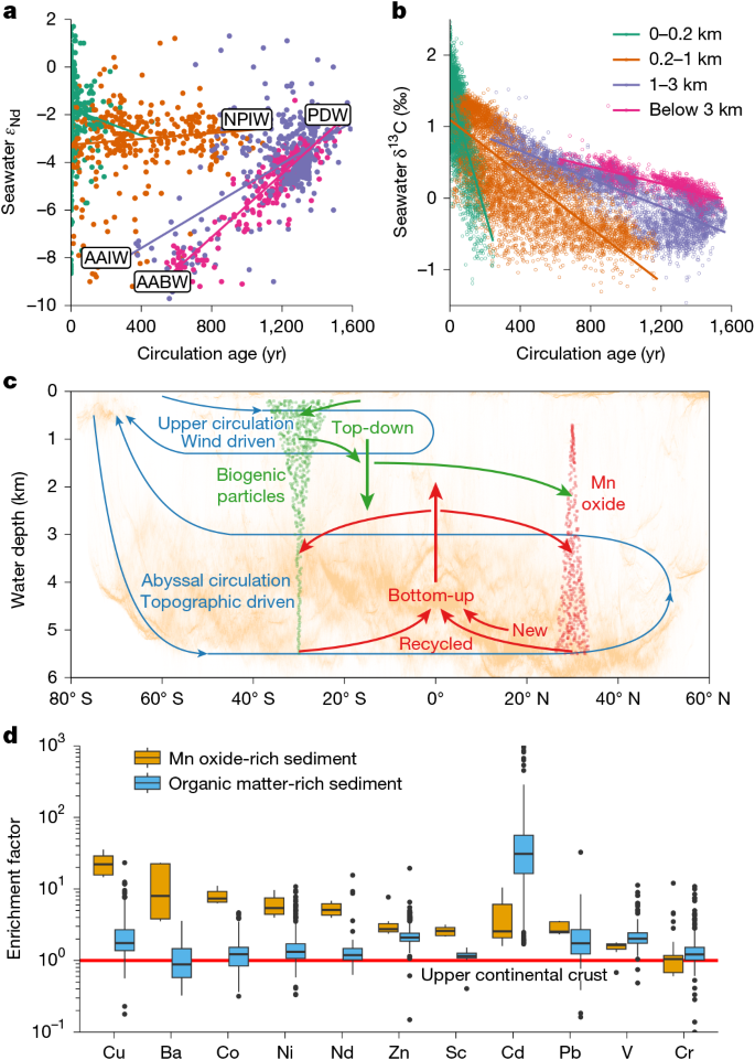
a,b, Comparing the bottom-up driven tracer ε_Nd (a) with the top-down driven tracer δ¹³C (ref. ⁵⁸; b). The non-conservativity of ε_Nd is higher in the abyssal ocean whereas for δ¹³C it is the greatest at the surface ocean. Compiled seawater data are colour-coded by the depth range. Major Pacific water masses are shown in the plot, including Antarctic bottom water (AABW), Antarctic intermediate water (AAIW), Pacific deep water (PDW) and North Pacific intermediate water (NPIW). c, Conceptual model of bottom-up versus top-down biogeochemical cycles. The background colour is the distribution of the seafloor area in ETOPO 2022⁵⁷. The cycling of a top-down tracer mainly consists of surface uptake and regeneration in the upper ocean. The cycling of a bottom-up tracer is dominated by benthic processing that largely happens on the oxic abyssal seafloor. The top-down and bottom-up processes are linked by particle production and scavenging. The affinity to biogenic versus oxide particles controls the relative importance of top-down and bottom-up processes in a tracer’s distribution. A tracer’s biogeochemical cycle is strongly tied to ocean circulation, which controls the preformed properties and dictates the exposure time to water-column and benthic processing. d, Affinity of selected trace elements to authigenic oxides compared with that to organic matter. The affinity is shown using elemental enrichment factors in oxide-rich sediments (this study) and organic-rich sediments⁴⁹ (greater than 2 wt% organic carbon content), calculated as metal-to-aluminium-concentration ratio in sediment relative to that in the upper continental crust⁴¹. The red line indicates no enrichment. In the boxplot, boxes show the interquartile range; thick lines show the median; whiskers extend to 1.5 × interquartile range away from the boxes; dots are outliers.

Our model further highlights the importance of particle-type-dependent scavenging. How strongly a trace metal is partitioned into oxides versus biogenic particles is a key control over its distribution. We qualitatively evaluate this relative affinity by comparing the enrichment factors of trace metals in oxide-rich abyssal sediments with those in organic-rich sediments⁴⁹ (Fig. 5d). Contrary to REE, for example, cadmium (Cd) appears to represent an endmember that strongly favours association with organic matter, consistent with its water-column profile being the most nutrient-like among trace elements²¹. Copper, colbalt, nickel and zinc are bio-essential, but they also have a high affinity for Mn oxide. Accordingly, elements like Cu should have scavenged-type water-column profiles, but are actually observed to increase linearly⁵⁰, like Nd. Our framework thus predicts that there is strong benthic flux of Cu from abyssal sediment, a prediction supported by observations and models^19,20,31.

We argue that the benthic impact is widespread among trace metals based on existing porewater data from the abyssal seafloor^19,20, and draw attention to some key implications for using TEIs in tracing ocean processes.

First, marine silicate weathering can provide a new source of trace elements and thus may explain disparities in isotopic budgets of some marine metals¹⁴. For Fe and Nd, this appears to be a robust conclusion^6,8,15,28, and similar arguments have been made for Cu (ref. ⁵⁰). Beyond a better understanding of tracers, marine silicate weathering may consume as much carbon dioxide as continental silicate weathering⁵¹. Our model provides a foundation to re-evaluate the role of silicate weathering, no longer a strictly continental phenomenon^52,53, as a buffering agent of climate change and a driver of ocean biogeochemical evolution.

Second, deep-ocean processes, such as hydrothermalism and oxygenation, affect the global ocean budgets of trace elements. For example, hydrothermalism today is the dominant source of both dissolved seawater Mn and thus of particulate Mn oxide⁵⁴ (Fig. 3c,d and Extended Data Fig. 6). Our model shows that variations in Mn-oxide cycling will exert strong control over trace-metal behaviours (Fig. 3b), even those that are not traditionally seen as sensitive to hydrothermalism and redox⁵⁵. Our model thus offers a different way of understanding and interpreting a wide range of ocean tracers with respect to hydrothermalism, ventilation and the redox nature of the deep sea.

Finally, our model places emphasis on the geometry of the ocean basins via its impact on abyssal mixing and circulation¹⁷. For example, today, bottom-intensified mixing is concentrated near mid-ocean ridges¹⁷, and thus the average depth of the crest (about 2.5 km) delineates the vertical reach of the abyssal sedimentary imprint (Fig. 5c). Few, if any, OBMs have investigated the biogeochemical impact of topographic mixing. We argue that the evolution of palaeobathymetry will be important in better understanding of the long-term history of ocean biogeochemistry.

Particle scavenging

We quantitatively partitioned scavenged Nd into fractions associated with each particle type. First, we estimated the particle-specific partition coefficients of Nd. Assuming reversible scavenging, the concentration of scavenged Nd (Nd_s) is:

where i is the index of particle type, including Mn oxide, Fe oxide, POM, calcium carbonate (CaCO₃), opal and lithogenic particle, \({K}_{{\rm{d}}}^{i}\) and Cⁱ are the apparent partition coefficient and particle concentration of the ith particle type, and Nd_d is the total dissolved Nd concentration. Here we assume that \({K}_{{\rm{d}}}^{i}\) is a constant, a standard practice in the literature^24,39. When using the total dissolved concentration in equation (1), \({K}_{{\rm{d}}}^{i}\) is an apparent constant, as in principle it should depend on metal speciation⁵⁹. Given the relative uniformity of deep-ocean properties, it is reasonable to assume that speciation in seawater is roughly the same and treat \({K}_{{\rm{d}}}^{i}\) as a constant. However, in pore water, speciation can strongly differ from seawater and changes with sediment depth; it is thus preferable to model \({K}_{{\rm{d}}}^{i}\) as a variable (see below).

Equation (1) is rewritten following refs. ^24,39:

where TP is the total particle concentration, \({K}_{{\rm{d}}}^{{\rm{TP}}}\) is the total particle partition coefficient and fⁱ is the mass fraction of the ith particle type.

We used data from the GEOTRACES Pacific GP16 and Atlantic GA03 cruises to characterize the particle scavenging of Nd (refs. ^25,38,60,61). These are so far the only cruises reporting both dissolved and particulate Nd data, as well as necessary bulk particulate data to carry out this analysis. The particulate data were size-fractionated (small particle, about 1–51 μm; large particle, >51 μm). Here we assume that K_d is not size specific. The GEOTRACES dissolved and particle samples were collected using Niskin bottles and McLane pumps, respectively, and thus are from slightly different depths. To create a paired dataset, we interpolated the dissolved Nd concentration at the depths of the particulate data.

The concentration of scavenged Nd is calculated by removing the lithogenic background from the measured total particle Nd concentration. In the original studies^25,60, titanium (Ti) and aluminium (Al) were used for detrital correction of the Atlantic GA03 and Pacific GP16 data, respectively, to estimate the concentrations of lithogenic particle and authigenic Fe oxide and Mn oxide. To be consistent, we also used Ti and Al for detrital correction of Nd at the GA03 and GP16 sites, respectively, assuming that the detrital Nd/Ti or Nd/Al ratio is the same as the upper continental crust⁴¹.

Equation (2) forms a system of equations that we solved for \({K}_{{\rm{d}}}^{i}\) using least-square estimation. To ensure the non-negativity of \({K}_{{\rm{d}}}^{i}\), the estimation was performed in terms of \({\log }_{10}{K}_{{\rm{d}}}^{i}\). We used a global black-box optimization method with constraints (ranges of \({\log }_{10}{K}_{{\rm{d}}}^{i}\) were set to −10 to 10) from the Julia package BlackBoxOptim.jl⁶². To account for data heterogeneity and provide error estimates, we performed the estimation 1,000 times by randomly sampling 75% of the data each time. When all particle data were used, the estimation gave \({\log }_{10}{K}_{{\rm{d}}}^{i}\) values of 8.66 (median, 8.63 to 8.72 interquartile range), 7.21 (7.17 to 7.26), 5.55 (5.10 to 5.81), 6.12 (5.92 to 6.22), −2.33 (−9.53 to 5.38) and −9.53 (−9.79 to −9.24) for Mn oxide, Fe oxide, POM and CaCO₃, lithogenic particles and opal, respectively. This shows that lithogenic particles and opal are negligible scavengers of Nd, consistent with the observation that \({K}_{{\rm{d}}}^{{\rm{TP}}}\) has no statistically significant (P > 0.1) relationship with lithogenic particles and opal fⁱ. However, if we restrict the particle data to below the surface (>200 m), our estimate shows that \({\log }_{10}{K}_{{\rm{d}}}^{i}\) of Mn oxide, Fe oxide and POM still have narrowly defined distributions overlapping with the aforementioned estimates, but \({\log }_{10}{K}_{{\rm{d}}}^{i}\) of CaCO₃ has a bimodal distribution with a wide interquartile range of −8.93 to 6.07 (median of 5.74), consistent with the observation that the correlation of \({K}_{{\rm{d}}}^{{\rm{TP}}}\) with \({f}^{{{\rm{CaCO}}}_{3}}\) is statistically insignificant (P > 0.1) below the surface. This result shows that CaCO₃ may be an important scavenger of Nd in the surface ocean but not at depth. Alternatively, this disparity may be the result of neglecting aqueous speciation when estimating \({K}_{{\rm{d}}}^{i}\), considering that seawater Nd exists mainly as carbonate complex and the carbonate speciation differs between the surface and deep⁵⁹. We are mainly interested in particle scavenging beneath the surface. Thus, we ignore the contribution of CaCO₃ to Nd scavenging in Fig. 1. However, to be comparable with previous reversible scavenging models, we included model sensitivity experiments where we allowed scavenging onto opal and CaCO₃, as discussed later. Finally, we performed an estimation including only oxides and POM. The estimated \({\log }_{10}{K}_{{\rm{d}}}^{i}\) and associated uncertainty of this final analysis are reported in the main text.

Our result of the varying affinity of Nd with particle types are consistent with previous field and laboratory studies. Chemical extractions of the labile proportion of marine particles have REE patterns that resemble that of the Mn oxide^11,63. Aqueous and surface complexation modelling have suggested that in the deep ocean, the dissolved seawater REE patterns are most likely explained by scavenging onto Mn oxide⁵⁹. In contrast, it has long been known that pristine biogenic carbonate contains little REE⁶⁴, and the REE associated with planktic foraminifera are predominantly hosted by oxides attached to the shell rather than within biogenic carbonate⁶⁵. Moreover, sediment-trap studies have found that settling biogenic opal does not contain a resolvable amount of LREE (although it may contain some HREE)⁶⁶. The evidence all points to Mn oxide as the dominant REE scavenger, particularly in the deep ocean, whereas the roles of biogenic carriers, especially carbonate and opal, are negligible.

Pacific cruise

We collected water-column, sediment and porewater samples during the KM2012 cruise (October 2020) onboard R/V Kilo Moana at 3 sites from the equatorial North Pacific along 152° W (Station 3, 11° N, 5,388 m; Station 4, 3° N, 5,050 m; Station 5, 7° N, 5,502 m). Sampling procedures followed ref. ⁴⁴ and are briefly summarized here. Water-column samples were collected and filtered (<0.45 μm) from Niskin bottles on a CTD Rosette. Sediment cores were collected using an MC800 multi-corer and sectioned at 1.2-cm intervals. Porewater aliquots for REE concentration and ε_Nd were collected by centrifuge and filtration (<0.45 μm). The REE aliquots were extracted from one core, and the ε_Nd aliquots combined extractions from corresponding layers of 20 to 25 cores. The REE aliquots include porewater samples from the top 20 cm and all seawater samples from each station, whereas the ε_Nd aliquots are fewer, having only porewater samples from the top 10 cm and the 3 bottom-most seawater samples at each station. Porewater aliquots for nutrient analyses were extracted using Rhizon samplers and filtered (<0.2 µm). Porewater aliquots for dissolved organic carbon (DOC) analysis were extracted via Rhizon, filtered (<0.45 μm with GFF filter), and poisoned with mercuric chloride and stored in a glass vial. Porewater dissolved oxygen (O₂) concentration was measured using a fibre-optic oxygen microsensor inserted into pre-drilled holes through the core into the sediments. The sensor readings were converted to O₂ concentration by linearly calibrating against the published bottom-water O₂ concentration at the study sites. Porewater pH was measured on unfiltered samples using a portable pH sensor post-extraction via centrifugation. Analysis of pH in pore waters is notoriously difficult owing to the changes in pressure upon recovery, and thus the pH data have finite utility. Sediment samples were frozen onboard and freeze-dried in the lab.

Elemental concentrations of the REE aliquots were analysed at Oregon State University using an Elemental Scientific seaFAST-pico offline pre-concentration technique, and the procedure has been extensively documented as part of the GEOTRACES intercalibration effort⁶⁷. Elemental concentrations of the ε_Nd aliquots (approximately 10 ml) were analysed at ETH Zurich using Nobias Chelate-PA1 resin in a manual column procedure⁶⁸. The measured REE concentration and pattern from the two labs agree well (Fig. 2 and Extended Data Fig. 3), and the small differences are expected given that the REE and ε_Nd aliquots represent samples extracted from different cores. The porewater REE concentration of the REE aliquots measured at Oregon State University shows a deep peak between 10 cm and 15 cm, but the scatter in observations of this peak is large among the 3 sites (Fig. 2), despite similarities in the REE pattern between all samples analysed (Extended Data Fig. 3). Unfortunately, the ε_Nd aliquots did not extend to this interval and thus we were not able to confirm this feature at ETH Zurich. While inherently interesting, this deeper peak does not affect our estimation of the benthic flux, which depends on only the REE concentration data at the sediment–water interface. Thus, for the intention of this paper, we have omitted interpretation of this feature. Also, we do not discuss cerium (Ce) in this study, because of the large inter-lab disagreement shown in the GEOTRACES intercalibration effort⁶⁷, and its fractionation from other REE owing to redox sensitivity.

Isotope analysis of the ε_Nd aliquots (about 400–700 ml of pore water or about 1.5 l of seawater) were done at ETH Zurich. Samples were buffered to a pH of 5.5 ± 5 and pre-concentrated using an in-house extraction manifold containing Nobias Chelate-PA1 resin. The procedure has been extensively used for trace-metal isotope analysis at ETH Zurich^69,70. After pre-concentration, separation of Nd from the matrix elements and other REE was done using Eichrom RE and LN spec resins. Ultimately, about 5–10 ng of Nd was available for isotope measurements. Procedural blanks were <3 pg. Isotope analysis was done on a Neptune Plus multi-collector inductively coupled plasma mass spectrometer (Thermo Fisher) following the procedure of ref. ⁷¹. Internally normalized sample data were renormalized to the ¹⁴³Nd/¹⁴⁴Nd ratio of La Jolla⁷². Repeated analysis of 8-ppb La Jolla solutions results in a long-term external reproducibility of 0.27 ε (2σ). Nd isotope analysis was also quality-controlled by repeated measurements of the US Geological Survey reference materials BCR-2 (ε_Nd = −0.11 ± 0.25, 2σ) and BHVO-2 (ε_Nd = 6.70 ± 0.24, 2σ) at the same concentration (about 5–10 ppb) as the porewater samples in agreement with literature results⁷³.

Nutrients were analysed at Oregon State University using a Technicon AutoAnalyzer II (phosphate and ammonium) and an Alpkem RFA 300 (silicic acid, nitrate + nitrite). The method and data processing follow ref. ⁷⁴. DOC was analysed with a V-CSN/TNM-1 (Shimadzu) at the Scripps Institution of Oceanography following ref. ⁷⁵. Sediment samples were analysed for total organic carbon contents using a GVI (now Elementar) Isoprime 1000 with Eurovector EA at Bigelow Laboratory for Ocean Sciences. Samples were measured for the total carbon (organic plus inorganic) and a separate sample split was acidified to remove carbonate and then measured for the organic fraction. Freeze-dried bulk sediments were digested in a concentrated HCl–HNO₃–HF mixture at high pressure, using a microwave-assisted system (CEM MARS-6), and sediment elemental concentrations were measured using inductively coupled plasma optical emission spectroscopy and an inductively coupled plasma mass spectrometer at Oregon State University⁷⁶. X-ray diffraction of freeze-dried raw samples were made at K/T GeoServices, using a Siemens D500 automated powder diffractometer equipped with a Cu X-ray source (40 kV, 30 mA) and a scintillation X-ray detector. Semi-quantitative determinations of whole-sediment mineral amounts were done using Jade Software (Materials Data) with the Whole Pattern Fitting option. Estimation of sedimentation rate was done by radiocarbon dating planktic foraminiferal shells from Station 4 (W. M. Keck Carbon Cycle AMS Facility, UC Irvine), where enough carbonate is available.

Abyssal Pacific sediment

Save for the presence of considerable biogenic carbonates at Station 4 (30% to 73% calcite based on X-ray diffraction) compared with Station 5 (0%) and Station 3 (about 0–1.6%), the sediment mineralogy is similar at all sites, being composed of quartz (about 4–11%), plagioclase (about 3–10%) and illite + mica (about 6–15%), with lesser components of K-feldspar (about 0.7–4%) and chlorite (about 0.7–3%), assuming halite and gypsum reflect dried pore water. There is a large fraction of a semi-quantifiable amorphous phase at all sites (about 40%).

Dissolved oxygen and nitrate + nitrite indicate that aerobic respiration dominates organic-matter remineralization and that diffusion from seawater is sufficient to keep the sediment package oxygenated with no sign of denitrification or more reducing conditions within the upper 20 cm (Fig. 2). Consequently, porewater Fe and Mn was below our detection limits (0.1 μM) in all cores. This diagenetic setting is consistent with previous work in the area⁷⁷. The relatively low organic-matter rain rate⁷⁷ (about 0.1–0.4 mmol m⁻² d⁻¹) combined with aerobic respiration result in low concentrations of particulate (POC, about 0.4 wt% in the mixed layer and about 0.15 wt% below) and dissolved (DOC, about 200–400 μM close to the interface and about 100 μM below) organic matter (Fig. 2).

Authigenic enrichment of metals at the study sites were estimated using detrital correction with Ti assuming that the element/Ti ratio is the same as the upper continental crust⁴¹. Whether using Al or Ti for this correction makes little difference. For example, the estimated mean authigenic Nd concentration is 53 ppm using Al versus 51 ppm using Ti. There is little vertical change of elemental concentrations in the upper-sediment package because of bioturbation. The means of estimated authigenic Nd concentration in the upper 30 cm at Stations 3, 4 and 5 are 49 ± 5 ppm (1σ), 33 ± 7 ppm and 73 ± 9 ppm respectively, and the mean of all samples combined is 51 ± 18 ppm. This inter-site difference is entirely attributed to dilution by biogenic materials (mainly carbonate which is much higher at Station 4). The relative authigenic enrichment of Nd, expressed as the ratio of authigenic to total Nd, is nearly identical at all sites, and the mean ratio of all samples combined is 0.76 (±0.09, a relative standard deviation of about 10% which is comparable to analytical precisions). The result demonstrates a high degree of homogeneity of the authigenic sediments in the study region despite the strong surface-productivity gradient, consistent with biogenic particles contributing little to the particulate REE flux.

REE carriers

Geochemical data of water-column particles and oxide-rich sediment phases were compiled and compared with our abyssal authigenic sediments. The paired particle Nd, Mn and Fe data shown in Extended Data Fig. 1a are available only from the GEOTRACES studies^25,38,60. However, because few sites in the GEOTRACES dataset reported the full REE data, the particle REE data shown in Extended Data Fig. 1c mainly come from other literature sources^{11,63,78,79,80}. In these studies, water-column particulate authigenic REE concentrations were either reported using chemical extraction^11,63, or estimated here using detrital correction based on Al (ref. ⁷⁹) or Th (refs. ^38,78,80), depending on which measurement was available. The Mn–Fe crust and nodule data are from the National Oceanic and Atmospheric Administration and Minerals Management Service Marine minerals geochemical database⁸¹. The data of dispersed Mn–Fe oxides in marine sediments extracted by leaching sediments or foraminifera are compiled by ref. ⁴⁷. The K_d of water-column particles were computed using the estimated authigenic REE concentration and paired seawater dissolved REE concentration from the same study. When computing K_d for crusts and nodules, we used the REE concentrations of our Pacific bottom water to represent deep-ocean seawater in general. When computing K_d for the authigenic sediment, we used the estimated authigenic REE concentrations and bottom-water dissolved REE concentrations from our study sites. Finally, we also compared our data with the Pacific sediment compilation of ref. ⁸² when showing the correlation between Nd and Mn concentrations in abyssal sediments (Extended Data Fig. 1d).

Previous studies have shown that phosphate is also an important host of REE in abyssal sediments^82,83. This observation does not contradict our conclusion that oxides are the main carriers of REE in the water column and surface sediments. As pristine biogenic phosphates contain negligible amounts of REE⁶⁴, the association of REE with phosphates can only happen post-deposition. Studies have demonstrated the diagenetic transfer of REE from oxides to phosphates on the Oregon margin using diagenetic modelling¹⁵, and on the abyssal seafloor using geochemical and mineralogical analysis⁸⁴. Because this kinetic mass transfer is slow on the abyssal seafloor (>10⁴ years according to ref. ⁸⁴), the association with phosphate manifests more strongly in the deeper sediment package, and in regions of lower sedimentation rate⁸³. However, this mass transfer has little effect on the total solid sediment budget, and the total (oxide plus phosphate) authigenic REE burial flux remains similar to that of the oxide-carried particle rain rate¹⁵. For example, a much higher authigenic Nd concentration up to 300 ppm hosted in phosphate-rich abyssal sediments has been found in locations with a much lower sedimentation rate (<0.05 cm kyr⁻¹)⁸³, yet the implied burial rate is <40 pmol cm⁻² yr⁻¹, no more than at our sites and entirely supportable by the Mn oxide-hosted particle rain rate. Thus, we conclude that this diagenetic transfer reconciles the apparent dichotomy that scavenged REE reaching the abyssal seafloor is mainly hosted by Mn oxide, yet in deeply buried sediments phosphate can be the main carrier.

Water-column and sediment mass fluxes

Given the uniformity of authigenic enrichment and detrital mineralogy, we assume that the fluxes of the non-biogenic (detrital and authigenic) materials are similar at the three sites. Our estimation of sediment burial flux uses data from Station 4 where radiocarbon dating is possible. The data here show a bioturbated depth of about 9 cm and a burial velocity of 0.53 cm kyr⁻¹. The burial rate is computed as

where ϕ is porosity (0.85 ± 0.04, 1σ, assuming 5% uncertainty), ρ is sediment grain density (2.65 ± 0.13 g cm⁻³, assuming 5% uncertainty), w is the burial velocity (0.53 ± 0.077 cm kyr⁻¹), and M is the total (42 ± 1 ppm Nd) or authigenic (36 ± 1 ppm Nd) concentration in the mixed layer. Errors are propagated into the results.

To estimate the particle Nd rain rate, we combine the GEOTRACES particle concentration data²⁵ with the Joint Global Ocean Flux Study (JGOFS) particle flux data^85,86,87 based on sediment traps. The rain rate is computed as

where F_p is the particle flux and Nd_p is the total or authigenic Nd concentration in particles. The JGOFS equatorial Pacific traps were deployed along approximately 140° W (15° S–15° N), slightly eastwards of our study sites (152° W, 3° N–11° N). The particle mass flux measured by the traps below 3,000 m at 5° N (between our Stations 4 and 5) is 64 ± 16 mg m⁻² d⁻¹. The GEOTRACES GP16 Station 36 (152° W, 10.5° S) is the closest site with particulate data available that has an oceanographic setting similar to our sites²⁵. The total and authigenic Nd concentrations below 2,500 m (excluding the benthic nepheloid layer) in the sinking particles are 4.2 ± 1.3 ppm and 3.4 ± 1.2 ppm, respectively. The relative enrichment of authigenic Nd in the deep-ocean particles (about 80%) is similar to that in our abyssal sediments (about 76%).

Diagenetic model

We performed diagenetic modelling using SedTrace⁸⁸, a tool that automates the generation and simulation of trace-element diagenesis. The diagenetic equations of biogeochemical tracers and REE have been reported in our previous study of REE diagenesis on the Oregon margin¹⁵ as well as in the model description paper of SedTrace⁸⁸. The model includes the following biogeochemical tracers: POC, DOC, CaCO₃, O₂, NO₃, NH₄⁺, TCO₂ and H⁺. POC is modelled using a 2-G model, including a labial component (POC₁) and a refractory component (POC₂) suggested by previous works in the study region⁷⁷. We assumed that the POC components are first converted to DOC (DOC₁ and DOC₂ respectively), which subsequently undergo aerobic remineralization⁸⁹. We also included nitrification and carbonate dissolution in the model¹⁵. The pH model follows the standard construction in SedTrace⁸⁸.

The biogeochemical model is tuned to fit the average sediment biogeochemistry represented by Station 5 (Fig. 2). To capture the high concentration of DOC at the sediment–water interface (Fig. 2d), the labial DOC₁ (Extended Data Fig. 2b) needs to be a high-molecular-weight compound with low molecular diffusivity⁹⁰ relative to the refractory DOC₂, consistent with the conceptual model of POC remineralization in marine sediments⁸⁹. Because the abyssal sediment is poorly buffered, modelled pH decreases from 7.7 at the sediment–water interface to 7.2 at 20 cm, qualitatively consistent with the measured values (about 7.2–7.3 at Station 5, although we note the limited utility of this data because of the sampling issue mention above; Extended Data Fig. 2c).

Three processes affect porewater REE in the model: complexation with dissolved ligands, release during POM remineralization and sorption onto oxides. Complexation of REE with inorganic ligands and the related stability constants follow that of refs. ^59,91. We also include REE complexation with the two types of DOC, and the stability constants are tuned within the range of organic ligands reported in literature⁹² (Extended Data Fig. 3c). To model Nd by POM remineralization, we derive a reasonable estimate of the Nd/C ratio released by POM. We start from the water-column K_d of POM estimated above, and find a value that is consistent with this K_d and reasonably fits the porewater Nd profile. The release of the other REE is scaled to Nd, the REE pattern of which is tuned following the pattern of K_d of POM reported in the literature^93,94,95 (Extended Data Fig. 3b). Finally, we implement pH-dependent sorption of REE onto Mn–Fe oxides following refs. ^59,96,97, which was derived using laboratory adsorption experiments using synthetic oxides in ionic media similar to seawater. We assume that only the free REE ions are adsorbed, and use the pH-dependent free-ion-based \(\genfrac{}{}{0ex}{}{{\rm{f}}}{}{K}_{{\rm{d}}}\), which is related to the total concentration-based K_d:

where ^fα is the fraction of free ion. K_d is an apparent constant that depends on the speciation of REE. We estimated \(\genfrac{}{}{0ex}{}{{\rm{f}}}{}{K}_{{\rm{d}}}^{{\rm{N}}{\rm{d}}}\) using the \(\genfrac{}{}{0ex}{}{}{}{K}_{{\rm{d}}}^{{\rm{N}}{\rm{d}}}\) derived from the GEOTRACES particle data and seawater speciation results, and found that it is about three orders of magnitude higher than the experimental values measured using synthetic Mn–Fe oxides in the lab, a known discrepancy⁹⁸ that is likely attributed to the difference in the surface chemistry between natural and synthetic oxides and the uncertainty in the aqueous speciation of REE in seawater⁵⁹. In an ad hoc approach, we used the lab-based REE pattern of \(\genfrac{}{}{0ex}{}{{\rm{f}}}{}{K}_{{\rm{d}}}\) in the model, but scaling them such that the value of \(\genfrac{}{}{0ex}{}{{\rm{f}}}{}{K}_{{\rm{d}}}^{{\rm{N}}{\rm{d}}}\) is consistent with the field data. That our model can successfully reproduce the porewater data REE pattern suggests that although the lab-based values of synthetic oxide \(\genfrac{}{}{0ex}{}{{\rm{f}}}{}{K}_{{\rm{d}}}\) may not apply to natural oxides, their REE pattern appears like natural oxides. This implies that the discrepancy is caused by factors common to all REE, and thus most likely related to particle surface chemistry rather than REE speciation. To model porewater ε_Nd we added ¹⁴⁴Nd and the radiogenic ¹⁴³Nd as two individual tracers to the model¹⁵, both of which are subject to the same processes.

The decrease of pH reduces \(\genfrac{}{}{0ex}{}{{\rm{f}}}{}{K}_{{\rm{d}}}\), whereas the increase of organic ligand concentration lowers ^fα, thus decreasing K_d in sediment (Extended Data Fig. 2d), promoting relative desorption of REE from Mn–Fe oxides. Modelled REE speciation is shown using Nd and Lu to represent LREE and HREE, respectively (Extended Data Fig. 2e,f). K_d computed using equation (5) is shown in Extended Data Fig. 3a where the ribbon indicates the range of K_d in the sediment package. Modelled porewater REE patterns are shown by normalizing to either the local bottom water or Post-Archaean Australian Shale (PAAS) (Extended Data Fig. 3).

Benthic fluxes

The benthic flux of REE is calculated as:

where i is the index of REE species, including the inorganic species and complexes with DOCs, \({D}_{{\rm{sw}}}^{i}\) is the molecular diffusivity and ∂Cⁱ/∂z is the concentration gradient. The benthic flux is computed by summing over the individual species because the organic and inorganic ligands have different molecular diffusivity⁸⁹. This calculation is straightforward in the model as the individual species are modelled directly. For data-based estimates, we distinguish the low-diffusivity DOC₁ from the other species that have the same diffusivity in the model. The porewater concentration profiles of REE can be considered as the superposition of a shallow peak (DOC₁ complex) onto a slowly increasing background (DOC₂ and inorganic species) concentration. We use the concentration immediately below the shallow peak to represent the background concentration, and the concentration of the DOC₁ complex is calculated by subtracting the background from the measured profiles. ∂Cⁱ/∂z was then computed using the decomposed profiles. Given the small role of DOC₁ complexation in the speciation of LREE, Nd is negligibly affected by this decomposing compared with HREE Lu. The data-based estimate was done using the mean concentration profile averaged over the three sites, and the errors are propagated throughout the calculation to give an overall estimate of benthic flux and its uncertainty in the study region.

Aside from measured and modelled benthic REE fluxes, in Extended Data Fig. 3 we also show the following sedimentary fluxes: data-based total sediment and authigenic REE burial fluxes, and POM-associated REE rain rates used in the model.

Water-column model

We model the 3D distributions of Nd concentration using the transport matrix method^34,99:

where Nd_T is the total Nd concentration, and the dissolved (Nd_d) and scavenged Nd (Nd_s) are computed using equation (1) assuming reversible scavenging; T_c and T_w are the transport matrices for 3D ocean circulation and vertical particle sinking respectively; and F_river, F_dust and F_benthic are the per volume sources of Nd due to river input, dust deposition and benthic flux, respectively. Other sources are considered minor and not included^9,13,34,100. We create and solve the steady-state model using the Julia language package AIBECS.jl⁹⁹, which is similar to the popular AWESOME OCIM framework of ocean biogeochemical modelling¹⁰¹. Our model is inspired by previous models of marine Nd cycles^3,13,100,102, especially GNOM³⁴, but diverge from them in the implementation of the particle scavenging and benthic fluxes, as described in this study. We give a brief description of our model construction and experiments here.

The Ocean Circulation Inverse Model (OCIM)^43,103 has been widely used as the circulation matrix T_c in OBMs of trace elements^34,101. Here we use the OCIM2-48L version (2° horizontal resolution, 48 vertical layers), which updates the previous versions by adding more depth layers and implementing bottom-intensified mixing following the state-of-the-art parameterization of ref. ¹⁶. The result is a better representation of the abyssal Pacific circulation strongly shaped by seafloor topography⁴³, making this model version ideal for studying the bottom-up control on the marine Nd cycle.

Dissolved, scavenged and total Nd concentrations are related via K_d (equation (1)). In our model, we only include biogenic particles and MnO₂. We obtained a 3D field of POM from previous OBMs¹⁰¹ and mapped it onto the model grid. We obtained 3D fields of carbonate and opal concentrations using satellite-derived surface export flux and depth-dependent attenuation laws following previous models (remineralization length scales were set to 3,500 m for carbonate and 10,000 m for opal)^13,104.

We currently lack a faithful reconstruction of the 3D field of MnO₂ by OBMs owing to the challenge of modelling the marine Mn cycle⁵⁴. Instead, we use an artificial neural network (ANN) to interpolate the GEOTRACES particle data (IDP 2021 Version 2)³⁸ onto our model grid, as previous studies have done for other ocean biogeochemical fields^31,105. The data are mainly from the Pacific (GP16) and Atlantic (GA01, 03, 06), with minor contributions from Arctic (GN01, 02, 03) and Southern Ocean (GA10) cruises. This ANN is a perceptron consisting of 2 hidden layers with 50 neurons and rectified linear unit activation function. We train with the following predictors: sampled water depth and latitude; temperature, salinity, oxygen, phosphate and silicate concentrations from World Ocean Atlas⁵⁶; mixed-layer depth, Δ¹⁴C, POM concentration and ³He/⁴He ratio from previous OCIM studies^43,101,103; and transmissometer-derived nepheloid-layer particle concentration^101,106. These predictors are selected to account for potential locational, physical and biogeochemical factors controlling the distribution of MnO₂, as well as the influence of a hydrothermal source and sediment resuspension. The gridded data products of these predictors are interpolated at the GEOTRACES sample locations and model grid points. We randomly selected 80% of the data from each ocean basin to create a training dataset, and the residual 20% was used for testing. In this way, the ANN results are less biased towards any individual ocean basin. Such data partitioning was repeated to generate a 500-member ensemble. We trained the ANN with the Adam optimizer and L₂ regularization using the Julia machine-learning package MLJ.jl¹⁰⁷. The model misfit generally stops changing after about 50 epochs, and we terminate the training after 100 epochs. The correlation coefficients between the predicted and observed MnO₂ are 0.92 and 0.90 (in the log-transformed space) for the training and testing sets, respectively (Extended Data Fig. 6). The root mean square errors are 0.25 µg l⁻¹ for both sets. The generated MnO₂ field correctly captures the main features in the GEOTRACES observation³⁸ including, for example, the hydrothermal plume, nepheloid layers and oxygen minimum zones in the Pacific GEOTRACES transect GP16²⁵, and the strong benthic nepheloid layer in the Northwest Atlantic^60,106 (Extended Data Fig. 6).

The river discharge in the model is derived from a global discharge model¹⁰⁸, and the river dissolved Nd concentration is from the observational dataset of ref. ¹⁰⁹. We assume a 30% removal of river Nd flux in the estuary^9,110. Dust depositional flux in the model is derived from a global dust model¹¹¹. We assigned a dust Nd concentration of 27 ppm (similar to the upper continental crust) and solubility of 2%, as in previous models^9,13.

We treated the benthic flux per unit area as a function of water depth (Fig. 3e) and tuned it within the range of the observations in the model experiments. The published benthic flux data are derived using porewater profiles^44,68 and generally consider only the diffusive fluxes, which may underestimate the total benthic flux by ignoring other transport mechanisms such as bio-irrigation and advection^15,68. Ocean models, even the improved OCIM2-48L, generally cannot entirely capture ocean bathymetry owing to limited resolution. We use the ETOPO 2022 global relief model to derive a subgrid bathymetry that better captures the distribution of the area-to-volume ratio in the real ocean⁹⁹, and allows the conversion of benthic flux per unit area to benthic flux per unit volume (Fig. 3e,f and Extended Data Fig. 7).

Through sensitivity tests (Fig. 3 and Extended Data Figs. 4 and 5), we evaluated the potential impact of particle scavenging and benthic flux on the distribution of Nd concentration in the Pacific. In the first experiment, we do not consider benthic flux and only include POM as a scavenger. We use a K_d of 10^5.8 for POM, within the range of our data-derived values, and a settling velocity of 2.0 m per day similar to Th-based estimates^{2,112,113,114,115}. Although our analysis of the GEOTRACE particle data do not support opal and carbonate as important Nd scavengers, we still chose to perform model tests to be comparable with previous reversible scavenging models. In these tests, we set the K_d to 10^7.0 and 10^5.6 for opal and carbonate, respectively, and these values were chosen to fit the surface Nd concentrations (Extended Data Fig. 4). In the second experiment, we further added MnO₂ scavenging with a K_d of 10^8.7 (Extended Data Fig. 6), according to our data-derived value, while keeping other parameters the same. In the last experiment, we further added a benthic flux while keeping other parameters the same. We used a vertical profile of benthic Nd flux per area that is consistent with observations, which is converted to flux per volume using the seafloor-area-to-volume ratio in the model subgrid bathymetry (Fig. 3e,f and Extended Data Fig. 7).

The model equation for radiogenic ¹⁴³Nd is similar to that of total Nd (equation (9)), except that the sources on the right-hand side are converted to sources of ¹⁴³Nd according to their isotope compositions. We obtain the ε_Nd of river input according to the gridded continental rock ε_Nd dataset of ref. ¹³. We map the ε_Nd of dust based on dust provenance^13,111.

Previous studies often used the gridded global sediment detrital ε_Nd map⁹ to represent benthic flux ε_Nd. However, it is well recognized that detrital sediment ε_Nd do not always represent the ε_Nd of benthic flux^9,13,33,47, which is sometimes dominated by a small fraction of reactive detritus, such as volcanic materials in the Pacific^14,15,33. Consequently, such models have difficulty in explaining Pacific seawater ε_Nd data¹³. Other studies have attempted to modify the detrital ε_Nd map to solve this problem³⁴, but such modifications are generally arbitrary, and not constrained by studies of sedimentary Nd cycling.

Here we parameterize the benthic flux ε_Nd following our present and previous^{8,15,33,47,116} observational and modelling studies of sediment diagenesis. In the Pacific, we partition the benthic flux used in the Nd concentration model above into a recycled component and a new component. The ε_Nd of the recycled flux is set to be the same as seawater ε_Nd at the bottom-most water-column grid above the seafloor. The ε_Nd of the new flux is set to be pure volcanic (+10 ε). We use this value for sedimentary volcanics as a starting point for our sensitivity test. Our model choice of the proportion of the new source (0–30%) was based on porewater and authigenic sediment data^15,116 (Fig. 4b). If we set the new source ε_Nd to lower (higher) values, the porewater and authigenic sediment data would simply require a greater (lower) proportion of the new source, but the net effect of the new flux would remain the same. There is no observational study of benthic flux ε_Nd in other ocean basins, so outside of the Pacific we set the benthic flux ε_Nd to be the same as detrital sediment ε_Nd compiled by ref. ⁹ (Extended Data Fig. 8). Previous research has shown that using detrital ε_Nd to represent benthic flux ε_Nd works reasonably well in the other basins¹³. Our model results that the Southern Ocean ε_Nd can be reproduced (Fig. 4) shows that this approach is adequate given our focus on the Pacific Ocean, and we leave the study of benthic fluxes for the future.

In a set of sensitivity tests, we set the new component to be 0%, 10%, 20% and 30% of total benthic flux, respectively (Extended Data Fig. 9). We use the modelled total Nd concentration from the third experiment in the concentration sensitivity test (Fig. 3b). We model the concentration of radiogenic ¹⁴³Nd, and compute the ε_Nd letting ¹⁴³Nd and ¹⁴⁴Nd sum to the modelled total Nd.

We also tested model sensitivity to where the new benthic flux is applied. In the test shown in Fig. 4, the new flux is added to all seafloor areas in the Pacific. In Extended Data Fig. 10a–c, we limit the new benthic flux to the margins up to water depths of 1,000 m, 2,000 m and 3,000 m, respectively. In Extended Data Fig. 10d–f, we restrict the new flux to the abyssal seafloor below 3,000 m, either in the entire Pacific, or only in the South Pacific, or everywhere except the dust province in the North Pacific where detrital sediment is predominantly composed of Asian dust⁴⁸. The areal extent of the North Pacific dust province is delimited by the contour of detrital sediment ε_Nd of −8 (Extended Data Fig. 8).

Finally, we model the water-mass age (that is, ideal age) following the original OCIM2_48L study⁴³. The modelled circulation age is used to show the impact of benthic exposure time³³ on the distribution of seawater ε_Nd.

Bottom-intensified mixing

The diapycnal diffusivity κ_ρ in Extended Data Fig. 7c is computed using the state-of-the-art parameterization of topographic mixing driven by internal tide dissipation from ref. ¹⁶, which has been validated against microstructure observations. The horizontal mean depth profile is:

where B is buoyancy flux, N is buoyancy frequency, ε is turbulence production and ⟨⟩ denotes these are horizontally averaged. The diapycnal diffusion length of Nd is then:

The diffusion length L_Nd (Extended Data Fig. 7d) should be interpreted as the length scale that a source of Nd can be of influence by turbulent diffusion alone in the water column on the timescale of Nd residence time (τ_Nd). Literature reports of τ_Nd are in the range of about 350–750 years^{3,9,34,44,102,117}, and we use a value of 400 years as a first-order estimate.

Nd data compilation

We compiled literature data of seawater, core-top authigenic and detrital sediment ε_Nd, and seawater Nd concentration previously⁹, which is updated here to include recent GEOTRACES results^23,38,118 (Extended Data Fig. 8). The paired authigenic and seawater data shown in Fig. 4b were created by binning the Pacific data into boxes that have 10° latitudinal, 20° longitudinal and 300 m (about 0–1,500 m) or 1,000 m (below 2,000 m) vertical resolutions. Data that fall into the same box were averaged and the standard deviations are reported (Fig. 4b).

We also compiled Nd concentration data in organic-rich sediments from the literature^{55,116,119,120,121} to complement other trace-metal data from ref. ⁴⁹, shown in Fig. 5d.

The geochemical data generated by this study are available at the Biological and Chemical Oceanography Data Management Office (https://doi.org/10.26008/1912/bco-dmo.928400.1, https://doi.org/10.26008/1912/bco-dmo.928152.1, https://doi.org/10.26008/1912/bco-dmo.928246.1). GEOTRACES data are available at British Oceanographic Data Centre (https://doi.org/10.5285/cf2d9ba9-d51d-3b7c-e053-8486abc0f5fd). ETOPO 2022 bathymetry is available from NOAA National Centers for Environmental Information (https://doi.org/10.25921/FD45-GT74). Global tidal mixing data are available at https://doi.org/10.17882/73082. The NOAA and MMS Marine Minerals Geochemical Database is available at https://doi.org/10.7289/V52Z13FT. GLODAP (v2.2022) Pacific seawater δ¹³C data are available at https://doi.org/10.25921/1f4w-0t92. The global Nd data compilation is available at https://doi.org/10.5281/zenodo.10859057 (ref. ¹²²).

The source code of SedTrace is available on Zenodo at https://doi.org/10.5281/zenodo.7225861 (ref. ¹²³). The diagenetic model of REE is available on Zenodo at https://doi.org/10.5281/zenodo.10847073 (ref. ¹²⁴). The water-column Nd cycle model is available on Zenodo at https://doi.org/10.5281/zenodo.10847786 (ref. ¹²⁵).

References

Authors and Affiliations

1. Institute of Geochemistry and Petrology, Department of Earth and Planetary Sciences, ETH Zürich, Zürich, Switzerland

   Jianghui Du  (杜江辉), Jörg Rickli & Derek Vance

2. Key Laboratory of Orogenic Belts and Crustal Evolution, MOE; School of Earth and Space Sciences, Peking University, Beijing, China

   Jianghui Du  (杜江辉)

3. College of Earth, Ocean and Atmospheric Sciences, Oregon State University, Corvallis, OR, USA

   Brian A. Haley

4. Bigelow Laboratory for Ocean Sciences, East Boothbay, ME, USA

   James McManus

5. Institute of Earth Sciences, University of Lausanne, Lausanne, Switzerland

   Patrick Blaser

6. GEOMAR Helmholtz-Zentrum für Ozeanforschung Kiel, Kiel, Germany

   Patrick Blaser

Contributions

J.D. and B.A.H. were responsible for the conceptualization of this study. J.D. and B.A.H. led the interpretation of results with J.M., P.B. and D.V. B.A.H., J.M., J.D. and D.V. acquired the funding. B.A.H. and J.M. led the sample collection during the Pacific cruise. J.D., B.A.H. and J.M. generated the geochemical data with assistance from P.B. and J.R. using methods for Nd isotopes established by D.V. J.D. led the modelling and data synthesis with assistance from B.A.H. J.D. and B.H. wrote the paper with input from D.V., J.M., P.B. and J.R.

Corresponding authors

Correspondence to Jianghui Du  (杜江辉) or Brian A. Haley.

Competing interests

The authors declare no competing interests.

Peer review information

Nature thanks William Homoky and the other, anonymous, reviewer(s) for their contribution to the peer review of this work.

Open Access This article is licensed under a Creative Commons Attribution 4.0 International License, which permits use, sharing, adaptation, distribution and reproduction in any medium or format, as long as you give appropriate credit to the original author(s) and the source, provide a link to the Creative Commons licence, and indicate if changes were made. The images or other third party material in this article are included in the article’s Creative Commons licence, unless indicated otherwise in a credit line to the material. If material is not included in the article’s Creative Commons licence and your intended use is not permitted by statutory regulation or exceeds the permitted use, you will need to obtain permission directly from the copyright holder. To view a copy of this licence, visit http://creativecommons.org/licenses/by/4.0/.

Reprints and permissions

References

Anderson, R. F. GEOTRACES: accelerating research on the marine biogeochemical cycles of trace elements and their isotopes. Annu. Rev. Mar. Sci. 12, 49–85 (2020).
Bacon, M. P. & Anderson, R. F. Distribution of thorium isotopes between dissolved and particulate forms in the deep sea. J. Geophys. Res. Oceans 87, 2045–2056 (1982).
Siddall, M. et al. Towards explaining the Nd paradox using reversible scavenging in an ocean general circulation model. Earth Planet. Sci. Lett. 274, 448–461 (2008).
John, S. G. et al. The biogeochemical balance of oceanic nickel cycling. Nat. Geosci. 15, 906–912 (2022).
Weber, T., John, S., Tagliabue, A. & DeVries, T. Biological uptake and reversible scavenging of zinc in the global ocean. Science 361, 72–76 (2018).
Lacan, F. & Jeandel, C. Neodymium isotopes as a new tool for quantifying exchange fluxes at the continent–ocean interface. Earth Planet. Sci. Lett. 232, 245–257 (2005).
Haley, B. A., Du, J., Abbott, A. N. & McManus, J. The impact of benthic processes on rare earth element and neodymium isotope distributions in the oceans. Front. Mar. Sci. 4, 426 (2017).
Abbott, A. N., Löhr, S. C., Payne, A., Kumar, H. & Du, J. Widespread lithogenic control of marine authigenic neodymium isotope records? Implications for paleoceanographic reconstructions. Geochim. Cosmochim. Acta 319, 318–336 (2022).
Du, J., Haley, B. A. & Mix, A. C. Evolution of the global overturning circulation since the Last Glacial Maximum based on marine authigenic neodymium isotopes. Quat. Sci. Rev. 241, 106396 (2020).
Deng, K. et al. Dominance of benthic fluxes in the oceanic beryllium budget and implications for paleo-denudation records. Sci. Adv. 9, eadg3702 (2023).
Sholkovitz, E. R., Landing, W. M. & Lewis, B. L. Ocean particle chemistry: the fractionation of rare earth elements between suspended particles and seawater. Geochim. Cosmochim. Acta 58, 1567–1579 (1994).
Jeandel, C. Overview of the mechanisms that could explain the ‘boundary exchange’ at the land–ocean contact. Phil. Trans. R. Soc. A 374, 20150287 (2016).
Robinson, S. et al. Simulating marine neodymium isotope distributions using Nd v1.0 coupled to the ocean component of the FAMOUS–MOSES1 climate model: sensitivities to reversible scavenging efficiency and benthic source distributions. Geosci. Model Dev. 16, 1231–1264 (2023).
Jeandel, C. & Oelkers, E. H. The influence of terrigenous particulate material dissolution on ocean chemistry and global element cycles. Chem. Geol. 395, 50–66 (2015).
Du, J. et al. Reactive-transport modeling of neodymium and its radiogenic isotope in deep-sea sediments: the roles of authigenesis, marine silicate weathering and reverse weathering. Earth Planet. Sci. Lett. 596, 117792 (2022).
de Lavergne, C. et al. A parameterization of local and remote tidal mixing. J. Adv. Model. Earth Syst. 12, e2020MS002065 (2020).
de Lavergne, C., Madec, G., Roquet, F., Holmes, R. M. & McDougall, T. J. Abyssal ocean overturning shaped by seafloor distribution. Nature 551, 181–186 (2017).
Tagliabue, A. et al. Authigenic mineral phases as a driver of the upper-ocean iron cycle. Nature 620, 104–109 (2023).
Klinkhammer, G., Heggie, D. T. & Graham, D. W. Metal diagenesis in oxic marine sediments. Earth Planet. Sci. Lett. 61, 211–219 (1982).
Steiner, Z. et al. Trace element geochemistry in North Pacific red clay sediment porewaters and implications for water-column studies. Glob. Biogeochem. Cycles 37, e2023GB007844 (2023).
Bruland, K. W., Middag, R. & Lohan, M. C. in Treatise on Geochemistry 2nd edn (eds Holland, H. D. & Turekian, K. K.) 19–51 (Elsevier, 2014); https://doi.org/10.1016/B978-0-08-095975-7.00602-1.
Goldberg, E. D. Marine geochemistry 1. Chemical scavengers of the sea. J. Geol. 62, 249–265 (1954).
Basak, C. et al. Suspended particulate matter influence on dissolved Nd concentration and isotopic composition along GEOTRACES section GP16. Earth Planet. Sci. Lett. 635, 118692 (2024).
Hayes, C. T. et al. Intensity of Th and Pa scavenging partitioned by particle chemistry in the North Atlantic Ocean. Mar. Chem. 170, 49–60 (2015).
Lam, P. J. et al. Size-fractionated distributions of suspended particle concentration and major phase composition from the U.S. GEOTRACES Eastern Pacific Zonal Transect (GP16). Mar. Chem. 201, 90–107 (2018).
Lagarde, M., Pham, V. Q., Lemaitre, N., Belhadj, M. & Jeandel, C. Rare earth elements in the North Atlantic, part II: partition coefficients. Chem. Geol. 664, 122298 (2024).
Conway, T. M. & John, S. G. Quantification of dissolved iron sources to the North Atlantic Ocean. Nature 511, 212–215 (2014).
Homoky, W. B., John, S. G., Conway, T. M. & Mills, R. A. Distinct iron isotopic signatures and supply from marine sediment dissolution. Nat. Commun. 4, 2143 (2013).
Chen, M. et al. Boundary exchange completes the marine Pb cycle jigsaw. Proc. Natl Acad. Sci. USA 120, e2213163120 (2023).
Little, S. H. et al. Towards balancing the oceanic Ni budget. Earth Planet. Sci. Lett. 547, 116461 (2020).
Roshan, S., DeVries, T. & Wu, J. Constraining the global ocean Cu cycle with a data-assimilated diagnostic model. Glob. Biogeochem. Cycles 34, e2020GB006741 (2020).
Bruggmann, S., Severmann, S. & McManus, J. Geochemical conditions regulating chromium preservation in marine sediments. Geochim. Cosmochim. Acta 348, 239–257 (2023).
Abbott, A. N., Haley, B. A. & McManus, J. Bottoms up: sedimentary control of the deep North Pacific Ocean’s εNd signature. Geology 43, 1035–1035 (2015).
Pasquier, B. et al. GNOM v1.0: an optimized steady-state model of the modern marine neodymium cycle. Geosci. Model Dev. 15, 4625–4656 (2022).
Goldstein, S. L. & Hemming, S. R. in Treatise on Geochemistry (eds Holland, H. D. & Turekian, K. K.) 453–489 (Pergamon, 2003).
Du, J., Haley, B. A., Mix, A. C., Walczak, M. H. & Praetorius, S. K. Flushing of the deep Pacific Ocean and the deglacial rise of atmospheric CO2 concentrations. Nat. Geosci. 11, 749–755 (2018).
Homoky, W. B. et al. Iron colloids dominate sedimentary supply to the ocean interior. Proc. Natl Acad. Sci. USA 118, e2016078118 (2021).
GEOTRACES Intermediate Data Product Group The GEOTRACES Intermediate Data Product 2021 (IDP2021) (NERC EDS British Oceanographic Data Centre NOC, 2021); https://doi.org/10.5285/cf2d9ba9-d51d-3b7c-e053-8486abc0f5fd.
Tang, Y., Stewart, G., Lam, P. J., Rigaud, S. & Church, T. The influence of particle concentration and composition on the fractionation of 210Po and 210Pb along the North Atlantic GEOTRACES transect GA03. Deep Sea Res. I 128, 42–54 (2017).
Smith, C. R. et al. Latitudinal variations in benthic processes in the abyssal equatorial Pacific: control by biogenic particle flux. Deep Sea Res. II 44, 2295–2317 (1997).
Rudnick, R. L. & Gao, S. in Treatise on Geochemistry 2nd edn (eds Holland, H. D. & Turekian, K. K.) 1–51 (Elsevier, 2014).
Atkins, A. L., Shaw, S. & Peacock, C. L. Release of Ni from birnessite during transformation of birnessite to todorokite: implications for Ni cycling in marine sediments. Geochim. Cosmochim. Acta 189, 158–183 (2016).
Holzer, M., DeVries, T. & de Lavergne, C. Diffusion controls the ventilation of a Pacific shadow zone above abyssal overturning. Nat. Commun. 12, 4348 (2021).
Abbott, A. N., Haley, B. A., McManus, J. & Reimers, C. E. The sedimentary flux of dissolved rare earth elements to the ocean. Geochim. Cosmochim. Acta 154, 186–200 (2015).
Moore, W. S. et al. Enriched regions of 228Ra along the U.S. GEOTRACES Pacific meridional transect (GP15). J. Geophys. Res. Oceans 129, e2023JC020564 (2024).
Jones, K. M., Khatiwala, S. P., Goldstein, S. L., Hemming, S. R. & van de Flierdt, T. Modeling the distribution of Nd isotopes in the oceans using an ocean general circulation model. Earth Planet. Sci. Lett. 272, 610–619 (2008).
Du, J., Haley, B. A. & Mix, A. C. Neodymium isotopes in authigenic phases, bottom waters and detrital sediments in the Gulf of Alaska and their implications for paleo-circulation reconstruction. Geochim. Cosmochim. Acta 193, 14–35 (2016).
Nakai, S., Halliday, A. N. & Rea, D. K. Provenance of dust in the Pacific Ocean. Earth Planet. Sci. Lett. 119, 143–157 (1993).
Sweere, T., van den Boorn, S., Dickson, A. J. & Reichart, G.-J. Definition of new trace-metal proxies for the controls on organic matter enrichment in marine sediments based on Mn, Co, Mo and Cd concentrations. Chem. Geol. 441, 235–245 (2016).
Little, S. H. et al. Paired dissolved and particulate phase Cu isotope distributions in the South Atlantic. Chem. Geol. 502, 29–43 (2018).
Wallmann, K. et al. Silicate weathering in anoxic marine sediments. Geochim. Cosmochim. Acta 72, 2895–2918 (2008).
Isson, T. T. et al. Evolution of the global carbon cycle and climate regulation on Earth. Glob. Biogeochem. Cycles 34, e2018GB006061 (2020).
Torres, M. E. et al. Silicate weathering in anoxic marine sediment as a requirement for authigenic carbonate burial. Earth Sci. Rev. 200, 102960 (2020).
van Hulten, M. et al. Manganese in the west Atlantic Ocean in the context of the first global ocean circulation model of manganese. Biogeosciences 14, 1123–1152 (2017).
Fleischmann, S. et al. The nickel output to abyssal pelagic manganese oxides: a balanced elemental and isotope budget for the oceans. Earth Planet. Sci. Lett. 619, 118301 (2023).
Boyer, T. P. et al. World Ocean Atlas (NOAA National Centers for Environmental Information, 2018).
ETOPO 2022 15 Arc-Second Global Relief Model (NOAA National Centers for Environmental Information, 2022); https://doi.org/10.25921/FD45-GT74.
Olsen, A. et al. The Global Ocean Data Analysis Project version 2 (GLODAPv2)—an internally consistent data product for the world ocean. Earth Syst. Sci. Data 8, 297–323 (2016).
Schijf, J., Christenson, E. A. & Byrne, R. H. YREE scavenging in seawater: a new look at an old model. Mar. Chem. 177, 460–471 (2015).
Lam, P. J., Ohnemus, D. C. & Auro, M. E. Size-fractionated major particle composition and concentrations from the US GEOTRACES North Atlantic zonal transect. Deep Sea Res. II 116, 303–320 (2015).
Haley, B. A. et al. Rare earth element and neodymium isotopes of the eastern US GEOTRACES Equatorial Pacific zonal transect (GP16). Earth Planet. Sci. Lett. 576, 117233 (2021).
Feldt, R. BlackBoxOptim.jl. GitHub https://github.com/robertfeldt/BlackBoxOptim.jl (2024).
Bertram, C. J. & Elderfield, H. The geochemical balance of the rare earth elements and neodymium isotopes in the oceans. Geochim. Cosmochim. Acta 57, 1957–1986 (1993).
Shaw, H. F. & Wasserburg, G. J. Sm–Nd in marine carbonates and phosphates: implications for Nd isotopes in seawater and crustal ages. Geochim. Cosmochim. Acta 49, 503–518 (1985).
Tachikawa, K., Piotrowski, A. M. & Bayon, G. Neodymium associated with foraminiferal carbonate as a recorder of seawater isotopic signatures. Quat. Sci. Rev. 88, 1–13 (2014).
Akagi, T., Fu, F., Hongo, Y. & Takahashi, K. Composition of rare earth elements in settling particles collected in the highly productive North Pacific Ocean and Bering Sea: implications for siliceous-matter dissolution kinetics and formation of two REE-enriched phases. Geochim. Cosmochim. Acta 75, 4857–4876 (2011).
Behrens, M. K. et al. Rapid and precise analysis of rare earth elements in small volumes of seawater—method and intercomparison. Mar. Chem. 186, 110–120 (2016).
Deng, K., Yang, S., Du, J., Lian, E. & Vance, D. Dominance of benthic flux of REEs on continental shelves: implications for oceanic budgets. Geochem. Perspect. Lett. 22, 26–30 (2022).
Lemaitre, N., Du, J., de Souza, G. F., Archer, C. & Vance, D. The essential bioactive role of nickel in the oceans: evidence from nickel isotopes. Earth Planet. Sci. Lett. 584, 117513 (2022).
Vance, D. et al. The oceanic budgets of nickel and zinc isotopes: the importance of sulfidic environments as illustrated by the Black Sea. Phil. Trans. R. Soc. Math. Phys. Eng. Sci. 374, 20150294 (2016).
Vance, D. & Thirlwall, M. An assessment of mass discrimination in MC-ICPMS using Nd isotopes. Chem. Geol. 185, 227–240 (2002).
Thirlwall, M. F. Long-term reproducibility of multicollector Sr and Nd isotope ratio analysis. Chem. Geol. 94, 85–104 (1991).
Jochum, K. P. et al. GeoReM: a new geochemical database for reference materials and isotopic standards. Geostand. Geoanal. Res. 29, 333–338 (2005).
Gordon, L. I., Jennings, J. C. Jr, Ross, A. A. & Krest, J. M. A Suggested Protocol for Continuous Flow Automated Analysis of Seawater Nutrients (Phosphate, Nitrate, Nitrite and Silicic Acid) in the WOCE Hydrographic Program and the Joint Global Ocean Fluxes Study (WOCE Hydrographic Program Office, 1993).
White, M. E. et al. Refractory dissolved organic matter has similar chemical characteristics but different radiocarbon signatures with depth in the marine water column. Glob. Biogeochem. Cycles 37, e2022GB007603 (2023).
Muratli, J. M., McManus, J., Mix, A. & Chase, Z. Dissolution of fluoride complexes following microwave-assisted hydrofluoric acid digestion of marine sediments. Talanta 89, 195–200 (2012).
Hammond, D. E., McManus, J., Berelson, W. M., Kilgore, T. E. & Pope, R. H. Early diagenesis of organic material in equatorial Pacific sediments: stoichiometry and kinetics. Deep Sea Res. II 43, 1365–1412 (1996).
Garcia-Solsona, E. et al. Rare earth elements and Nd isotopes tracing water mass mixing and particle–seawater interactions in the SE Atlantic. Geochim. Cosmochim. Acta 125, 351–372 (2014).
Tachikawa, K., Jeandel, C., Vangriesheim, A. & Dupré, B. Distribution of rare earth elements and neodymium isotopes in suspended particles of the tropical Atlantic Ocean (EUMELI site). Deep Sea Res. I 46, 733–755 (1999).
Paffrath, R. et al. Seawater–particle interactions of rare earth elements and neodymium isotopes in the deep central Arctic Ocean. J. Geophys. Res. Oceans 126, e2021JC017423 (2021).
Grant, J. B., Moore, C. J., Alameddin, G., Chen, K. & Barton, M. The NOAA and MMS Marine Minerals Geochemical Database (NOAA National Geophysical Data Center, 1992); https://doi.org/10.7289/V52Z13FT.
Kato, Y. et al. Deep-sea mud in the Pacific Ocean as a potential resource for rare-earth elements. Nat. Geosci. 4, 535–539 (2011).
Deng, Y. et al. Early diagenetic control on the enrichment and fractionation of rare earth elements in deep-sea sediments. Sci. Adv. 8, eabn5466 (2022).
Takahashi, Y. et al. Transfer of rare earth elements (REE) from manganese oxides to phosphates during early diagenesis in pelagic sediments inferred from REE patterns, X-ray absorption spectroscopy, and chemical leaching method. Geochem. J. 49, 653–674 (2015).
Honjo, S., Manganini, S. J. & Cole, J. J. Sedimentation of biogenic matter in the deep ocean. Deep Sea Res. A 29, 609–625 (1982).
Honjo, S., Dymond, J., Collier, R. & Manganini, S. J. Export production of particles to the interior of the equatorial Pacific Ocean during the 1992 EqPac experiment. Deep Sea Res. II 42, 831–870 (1995).
Dymond, J. & Collier, R. Biogenic particle fluxes in the equatorial Pacific: evidence for both high and low productivity during the 1982−1983 El Niño. Glob. Biogeochem. Cycles 2, 129–137 (1988).
Du, J. SedTrace 1.0: a Julia-based framework for generating and running reactive-transport models of marine sediment diagenesis specializing in trace elements and isotopes. Geosci. Model Dev. 16, 5865–5894 (2023).
Burdige, D. J., Komada, T., Magen, C. & Chanton, J. P. Modeling studies of dissolved organic matter cycling in Santa Barbara Basin (CA, USA) sediments. Geochim. Cosmochim. Acta 195, 100–119 (2016).
Burdige, D. J., Alperin, M. J., Homstead, J. & Martens, C. S. The role of benthic fluxes of dissolved organic carbon in oceanic and sedimentary carbon cycling. Geophys. Res. Lett. 19, 1851–1854 (1992).
Schijf, J. & Byrne, R. H. Speciation of yttrium and the rare earth elements in seawater: review of a 20-year analytical journey. Chem. Geol. 584, 120479 (2021).
Lee, J. H. & Byrne, R. H. Examination of comparative rare earth element complexation behavior using linear free-energy relationships. Geochim. Cosmochim. Acta 56, 1127–1137 (1992).
Zoll, A. M. & Schijf, J. A surface complexation model of YREE sorption on Ulva lactuca in 0.05–5.0 M NaCl solutions. Geochim. Cosmochim. Acta 97, 183–199 (2012).
Byrne, R. H. & Kim, K.-H. Rare earth element scavenging in seawater. Geochim. Cosmochim. Acta 54, 2645–2656 (1990).
Freslon, N. et al. Rare earth elements and neodymium isotopes in sedimentary organic matter. Geochim. Cosmochim. Acta 140, 177–198 (2014).
Schijf, J. & Marshall, K. S. YREE sorption on hydrous ferric oxide in 0.5 M NaCl solutions: a model extension. Mar. Chem. 123, 32–43 (2011).
Marshall, K. The Influence of Iron and Manganese Oxides on the Production of Marine Sedimentary Cerium Anomalies. MSc thesis, Univ. Maryland (2011); http://drum.lib.umd.edu/handle/1903/12364.
Koeppenkastrop, D. & De Carlo, E. H. Sorption of rare-earth elements from seawater onto synthetic mineral particles: an experimental approach. Chem. Geol. 95, 251–263 (1992).
Pasquier, B., Primeau, F. W. & John, S. G. AIBECS.jl: a tool for exploring global marine biogeochemical cycles. J. Open Source Softw. 7, 3814 (2022).
Arsouze, T., Dutay, J.-C., Lacan, F. & Jeandel, C. Reconstructing the Nd oceanic cycle using a coupled dynamical—biogeochemical model. Biogeosciences 6, 2829–2846 (2009).
John, S. G. et al. AWESOME OCIM: a simple, flexible, and powerful tool for modeling elemental cycling in the oceans. Chem. Geol. 533, 119403 (2020).
Rempfer, J., Stocker, T. F., Joos, F., Dutay, J.-C. & Siddall, M. Modelling Nd-isotopes with a coarse resolution ocean circulation model: sensitivities to model parameters and source/sink distributions. Geochim. Cosmochim. Acta 75, 5927–5950 (2011).
DeVries, T. & Holzer, M. Radiocarbon and helium isotope constraints on deep ocean ventilation and mantle-3He sources. J. Geophys. Res. Oceans 124, 3036–3057 (2019).
Dunne, J. P., Hales, B. & Toggweiler, J. R. Global calcite cycling constrained by sediment preservation controls. Glob. Biogeochem. Cycles 26, GB3023 (2012).
John, S. G., Liang, H., Pasquier, B., Holzer, M. & Silva, S. Biogeochemical fluxes of nickel in the global oceans inferred from a diagnostic model. Glob. Biogeochem. Cycles 38, e2023GB008018 (2024).
Gardner, W. D., Jo Richardson, M., Mishonov, A. V. & Biscaye, P. E. Global comparison of benthic nepheloid layers based on 52 years of nephelometer and transmissometer measurements. Prog. Oceanogr. 168, 100–111 (2018).
Anthony Blaom, P. et al. alan-turing-institute/MLJ.jl: v0.20.3. Zenodo https://doi.org/10.5281/zenodo.10795902 (2024).
Müller Schmied, H. et al. The global water resources and use model WaterGAP v2.2 d: model description and evaluation. Geosci. Model Dev. 14, 1037–1079 (2021).
Goldstein, S. J. & Jacobsen, S. B. The Nd and Sr isotopic systematics of river-water dissolved material: implications for the sources of Nd and Sr in seawater. Chem. Geol. Isot. Geosci. Sect. 66, 245–272 (1987).
Tachikawa, K., Jeandel, C. & Roy-Barman, M. A new approach to the Nd residence time in the ocean: the role of atmospheric inputs. Earth Planet. Sci. Lett. 170, 433–446 (1999).
Kok, J. F. et al. Contribution of the world’s main dust source regions to the global cycle of desert dust. Atmos. Chem. Phys. 21, 8169–8193 (2021).
Roy-Barman, M., Chen, J. H. & Wasserburg, G. J. 230Th–232Th systematics in the central Pacific Ocean: the sources and the fates of thorium. Earth Planet. Sci. Lett. 139, 351–363 (1996).
Okubo, A., Obata, H., Gamo, T. & Yamada, M. 230Th and 232Th distributions in mid-latitudes of the North Pacific Ocean: effect of bottom scavenging. Earth Planet. Sci. Lett. 339–340, 139–150 (2012).
Lopez, G. I., Marcantonio, F., Lyle, M. & Lynch-Stieglitz, J. Dissolved and particulate 230Th–232Th in the central equatorial Pacific Ocean: evidence for far-field transport of the East Pacific Rise hydrothermal plume. Earth Planet. Sci. Lett. 431, 87–95 (2015).
Nozaki, Y., Horibe, Y. & Tsubota, H. The water column distributions of thorium isotopes in the western North Pacific. Earth Planet. Sci. Lett. 54, 203–216 (1981).
Abbott, A. N., Haley, B. A. & McManus, J. The impact of sedimentary coatings on the diagenetic Nd flux. Earth Planet. Sci. Lett. 449, 217–227 (2016).
Tachikawa, K., Athias, V. & Jeandel, C. Neodymium budget in the modern ocean and paleo-oceanographic implications. J. Geophys. Res. Oceans 108, 3254 (2003).
Waltemathe, H., Struve, T., Rehbein, M. & Pahnke, K. Influence of water mass mixing and hydrothermal processes on the distribution of dissolved Nd isotopes and concentrations in the South Pacific. Earth Planet. Sci. Lett. 642, 118846 (2024).
Orani, A. M. et al. Baseline study on trace and rare earth elements in marine sediments collected along the Namibian coast. Mar. Pollut. Bull. 131, 386–395 (2018).
Piper, D. Z. & Dean, W. E. Trace-Element Deposition in the Cariaco Basin, Venezuela Shelf, under Sulfate-Reducing Conditions: A History of the Local Hydrography and Global Climate, 20 Ka to the Present Professional Paper (USGS, 2002); https://doi.org/10.3133/pp1670.
Astakhov, A. S. et al. Distribution and sources of rare earth elements in sediments of the Chukchi and East Siberian seas. Polar Sci. 20, 148–159 (2019).
Du, J. Global data compilation of seawater, authigenic and detrital radiogenic neodymium isotope composition since the Last Glacial Maximum. Zenodo https://doi.org/10.5281/zenodo.10859057 (2020).
Du, J. SedTrace.jl: a Julia package for generating and running reactive-transport models of marine sediment diagenesis. Zenodo https://doi.org/10.5281/zenodo.7225861 (2023).
Du, J. Models of sediment diagenesis on the abyssal seafloor of the central North Pacific. Zenodo https://doi.org/10.5281/zenodo.10847073 (2025).
Du, J. Model of the water column Nd cycle in the Pacific. Zenodo https://doi.org/10.5281/zenodo.10847786 (2025).
Byrne, R. H. & Li, B. Comparative complexation behavior of the rare earths. Geochim. Cosmochim. Acta 59, 4575–4589 (1995).
Barth, A., Beckers, J.-M., Troupin, C., Alvera-Azcárate, A. & Vandenbulcke, L. divand−1.0: n-dimensional variational data analysis for ocean observations. Geosci. Model Dev. 7, 225–241 (2014).
Acknowledgements
We thank the captain, the crew and the scientific party during the KM2012 Pacific cruise onboard the R/V Kilo Moana; and J. Muratli and C. Archer for assistance with geochemical analysis. This project has received funding from the European Union’s Horizon 2020 research and innovation programme under the Marie Skłodowska-Curie grant agreement number 891489. J.D. was also supported by the National Key Research and Development Program of China (grant number 2024YFF0808000). Funding was also provided by the US NSF to B.A.H. (grant numbers 1850765 and 2148005) and to J.M. (grant number 1850789). P.B. acknowledges funding from the European Union’s Horizon Europe research and innovation programme (grant number 101065424, project OxyQuant) and the Swiss National Science Foundation (grant number 192361). The GEOTRACES 2021 Intermediate Data Product version 2 (IDP2021v2) represents an international collaboration and is endorsed by the Scientific Committee on Oceanic Research (SCOR). The many researchers and funding agencies responsible for the collection of data and quality control are thanked for their contributions to the IDP2021v2. This is a contribution from the PKU low-carbon metal group.
Funding
Open access funding provided by Swiss Federal Institute of Technology Zurich.
Ethics declarations