Age and gender distortion in online media and large language models

Although few deny that stereotypes, or generalizations about social groups^10,11,12, are harmful, a fundamental question remains contested: are common stereotypes accurate^1,2,3 or socially distorted^4,5,6? Some argue that commonplace stereotypes accurately capture observable aspects of social groups; otherwise, they would not gain such widespread adoption^1,2,3. Yet, others argue that stereotypes are often exaggerated or illusory^4,5,6. Assessing stereotype accuracy is challenging because stereotypes involve not only statistical associations (such as expected correlations among the features of a social group) but also normative judgements (such as that one group is superior to another) for which there is no well-defined ground truth^10,11,12. Even for statistical associations, identifying the ground truth is difficult. In some cases, this stems from disagreement on how to measure the ground truth, such as enduring debates over how to measure intelligence¹³ (a heavily stereotyped characteristic¹⁴). Yet, even when there is agreement on the relevant constructs, there is often a lack of large-scale, quantifiable cultural data for measuring stereotypical associations and comparing these to ground truth indicators. As a result, research on stereotypes often yields inconsistent findings, calling into question the pervasiveness and impact of these biases. In this study, we overcame these limitations in the analysis of age-related gender bias, which not only involves biological age as an objective anchor for evaluating stereotype accuracy, but which can also be linked to large-scale statistical biases in how the ages of women and men are depicted online.

On the one hand, evidence abounds that older women face a dual bias at the intersection of gender and age. Policy reports^8,15,16, media coverage¹⁷ and workplace interviews^7,18 indicate that older women are discriminated against in hiring and promotion across industries (known as ‘gendered ageism’^7,18,19). This is related to a general statistical bias towards associating women with expectations of youth. From entertainment media to the workplace, women face persistent pressure to appear young, which results in a ‘beauty tax’ with sizeable financial and time costs²⁰. This bias also manifests in everyday language. Women in academia²¹ and industry²² are more likely than men to be referred to using infantilizing pronouns (such as ‘girls’). These patterns suggest that age-related gender expectations may form a culture-wide statistical bias that influences people’s perceptions of others throughout society^23,24.

On the other hand, the statistical association between women and youth contradicts observable socioeconomic realities. Since the 1960s, women have consistently outlived men in the USA by as much as 8 years, a gap that has been increasing^25,26. Census data on occupations present similarly puzzling trends (Supplementary Fig. 1). Over the past decade, there has been no correlation between the fraction of women in an occupation and its median age, according to the US census (Extended Data Fig. 1 and Supplementary Table 1). There were also no clear differences in the age distribution of women and men throughout the workforce from 2009 to the present (Supplementary Fig. 2 and Supplementary Table 2). Moreover, recent surveys failed to observe gendered ageism in certain organizational settings and even suggest that older women may be less affected by stereotypes than older men^27,28. These inconsistent findings resonate with critiques against claims of enduring gender inequality, such as research showing declines in gender stereotypes over the last century in online text^29,30, as well as studies showing that hiring across industries increasingly favours women^31,32. This dissonant landscape raises the question of whether age-related gender bias is an organization-specific or industry-specific problem, or whether it is a culture-wide distortion that continues to reflect and contribute to systemic inequalities.

We argue that this uncertainty is fuelled by the lack of (1) culture-wide multimodal data on the associations between gender and age and (2) computational methodologies for comparing these associations with ground truth indicators. So far, only a handful of studies have examined age–gender associations in small-scale surveys and interviews with professional women^{7,18,27,28,33} or in sparse, non-representative observational studies of particular industries, such as celebrities and athletes in entertainment media^{34,35,36,37,38}. However, failing to observe age-related gender bias in limited samples of a few contexts does not indicate a lack of prominence on a culture-wide scale. Social biases in how people categorize the world frequently emerge only at scale^39,40 and can manifest as exaggerated or even illusory beliefs⁴¹. This suggests the alternative view that skewed associations between gender and age can emerge as a large-scale statistical bias that distorts socioeconomic realities despite inconsistencies across small-scale contexts.

Although a number of recent studies revealed the exaggeration of male representation in online texts and images^6,42, no comparable analyses exist for tracking age-related representations of gender. To address this gap, we produced a large-scale culture-wide dataset on age–gender associations across modalities, including images, videos and textual data, collected from popular sources of digital media. We began by examining the gender and age associations of all social categories in the English language (n = 3,495) in more than 1.3 million images and thousands of videos from Google, Wikipedia, IMDb, Flickr, YouTube and a random sample of the world-wide web (see ‘Image and video datasets’ in Methods for details on pre-processing and post-processing). We benchmarked online images of occupations against the US census data to examine whether they exaggerate the association between women and youth. We went beyond the visual modalities by examining age-related gender bias in nine popular language models trained on billions of words from across the internet, including Reddit, Google News, Wikipedia and Twitter (see ‘Measuring age and gender in online text’ in Methods). By examining age-related gender bias in large-scale internet data, our study was uniquely poised to examine the role that mainstream algorithms play in reinforcing this bias. We examined algorithmic amplification in both the image and textual modalities through (1) the study of the psychological effects of using Google Image search and (2) the use of ChatGPT to generate and evaluate resumes in the workplace.

Across all image datasets spanning five popular online platforms, women are consistently represented as younger than men, regardless of whether the age and gender of faces are measured using human judgements, machine learning or ground truth data. First, we analysed 657,035 images from the Google search engine associated with 3,495 social categories, in which the gender and age of images were classified by human coders⁶ (see ‘Image data collection procedure’ in Methods; all categories were examined using retrieved Google Images containing human faces). We found that women in Google Images were coded as significantly younger than men, both for non-gendered searches (such as ‘doctor’ or ‘banker’; mean difference in age groups, M_diff = 0.37; t = −73.84; P = 2.2 × 10⁻¹⁶; n = 3,434 categories; Fig. 1a) and gendered searches (such as searching ‘female doctor’ and ‘male doctor’; M_diff = 0.29; t = −36.52; P = 2.2 × 10⁻¹⁶; n = 2,960 categories; Fig. 1b). Replicating this method over Wikipedia revealed that women in Wikipedia images were also coded as significantly younger than men (M_diff = 0.71; t = −39.62; P = 2.2 × 10⁻¹⁶; n = 1,251 categories; Fig. 1c).

Fig. 1: Women are represented as significantly younger than men in more than 1.3 million images and thousands of videos across 7 online sources.

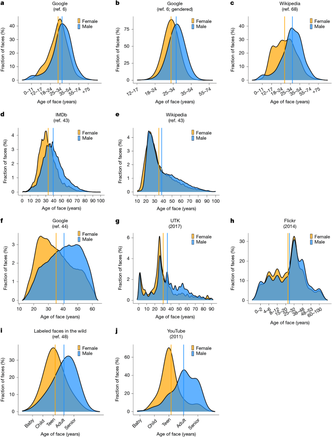
a–j, The age of either female or male faces according to the top 100 Google Images associated with 3,434 social categories (n = 161,484 images) (a), the top 100 Google Images retrieved using gendered searches (such as by searching ‘female athlete’ or ‘male athlete’) shown for all non-gendered categories in WordNet (n = 2,960 categories; 495,551 images) (b), 1,251 categories in Wikipedia (from the Srinivasan et al.⁶⁸ dataset; 14,709 images) (c), celebrities identified by the top 100,000 most popular pages on IMDb (n = 451,570 images) (d), biographical Wikipedia pages describing the same celebrities in the IMDb–Wiki dataset (n = 57,932 images) (e), the top 50 most popular celebrities from 1951 to 2004 as they appear in Google Images, according to the CACD (n = 149,889 images) (f), a random sample across the world-wide web (the 2017 UTK dataset; n = 20,000 images) (g), a random sample from Flickr (the 2014 Adience dataset; n = 26,580 images) (h), a random sample of images from online news websites (the 2008 LFW dataset; n = 13,233 images) (i) and images of the same people identified in the LFW dataset, extracted across 3,425 YouTube videos in 2011 (n = 5,000 images) (j). The method for coding age and gender varies by dataset; a–c rely on human coders; panels d,e,g rely on ground truth measures of the age and gender of celebrities posted publicly online; f,h–j rely on automated deep learning classifications of gender and age. Solid gold and blue lines indicate the average age for female and male faces, respectively.

These results are robust to collecting Google Images from different countries around the world (Supplementary Fig. 3) and controlling for (1) the demographic characteristics and subjectivity of human coders (Supplementary Figs. 4 and 5 and Supplementary Tables 3–5); (2) the linguistic features of social categories (Supplementary Figs. 6 and 7 and Supplementary Table 6), such as word polysemy, word gender connotation, word age connotation and word frequency in Google Search and in everyday language; (3) the visual features of the images, including the number of faces per image, the number of images associated with each category overall, whether the image repeats across searches and whether the image is photographic or displays a digital avatar (Supplementary Table 7); and (4) whether the faces in each image are cropped before classification (Supplementary Fig. 8), as well as statistical biases in the cropping algorithm itself (Supplementary Fig. 9). We confirm that these results reflect images from a wide range of websites (Supplementary Fig. 10).

Next, we analysed the 2018 IMDb–Wiki dataset⁴³ and the 2014 Cross-Age Celebrity Dataset (CACD)⁴⁴ consisting of Google Images, each of which provides the true gender and age of the celebrities depicted using their public bio pages and time-stamped photographs. Figure 1 shows that female celebrities are, on average, 6.5 years younger than men on IMDb (t = −169.9; P = 2.2 × 10⁻¹⁶; n = 451,562 images; Fig. 1d), 3.27 years younger on Wikipedia (t = 10.64; P = 2.2 × 10⁻¹⁶; n = 57,972 images; Fig. 1e) and 5.35 years younger in Google Images (t = −90.92; P = 2.2 × 10⁻¹⁶; n = 149,889 images; Fig. 1f). In all cases, the most common (modal) age for women is in their 20s, whereas in images from IMDb and Google, the most common ages for men are 40 years and 50 years, respectively. These analyses show that age-related gender bias online is not an artefact of human perceptions of gender and age, because it is replicated using verified objective information about the age and gender of those depicted. That age-based gender bias replicates strongly in the context of celebrities is concerning, given the salient role that celebrities play in reinforcing stereotypes⁴⁵.

Finally, we explored age biases in the representation of women and men using prominent image datasets developed for training machine learning algorithms. The age and gender classifications in these datasets were provided by computer vision algorithms constructed by the research teams that released these datasets. We found that women were automatically classified as significantly younger than men in the 2017 UTK⁴⁶ dataset consisting of a diverse sample of images from across the world-wide web (M_diff = 5.12 years; t = −19.9; P = 2.2 × 10⁻¹⁶; n = 24,106 images; Fig. 1g), the 2014 Adience dataset⁴⁷ consisting of images from Flickr (M_diff = 0.18; t = −6.52; P = 6.79 × 10⁻¹¹; n = 17,492 images; Fig. 1h) and the 2008 Labeled Faces in the Wild (LFW) dataset⁴⁸ consisting of a random sample of images from Google News (M_diff = 0.84; t = −44.89; P = 2.2 × 10⁻¹⁶; n = 13,143 images; Fig. 1i) (two-tailed Student’s t-test). These findings further generalized our results beyond the perceptions of human coders.

A remaining question is whether age-related gender bias is also observed in online videos, which increasingly dominate the world-wide web⁴⁹. Although an exhaustive analysis of online videos is beyond the scope of this study, we analysed two open-source datasets of screenshots from YouTube videos that provide compelling support for our theory. First, we examined the correlation between gender and age in the 2011 YouTube Faces dataset⁵⁰, consisting of 3,645 faces of celebrities extracted from 3,425 YouTube videos. Women in the YouTube Faces dataset appear significantly younger than men according to machine learning classifications (M_diff = 0.87; t = −25.68; P = 2.2 × 10⁻¹⁶; n = 3,645 images; Fig. 1j). We also analysed a more recent dataset of YouTube videos called the 2022 CelebV-HQ dataset⁵¹, consisting of 35,666 images collected by identifying public lists of celebrities on Wikipedia and automatically collecting the top 10 YouTube videos associated with each celebrity. Although this dataset contains only a binary measure of age (faces are coded as either young = 1 or old = 0), we can still test our theory by comparing the fraction of women and men coded as young. Only 20% of men were classified as young compared with 33% of women, marking a significantly higher rate of youthful presentations for women (P = 2.2 × 10⁻¹⁶; two-tailed proportion test).

A natural suspicion is that age-related gender bias in online images and videos may be driven by affordances of visual communication, such as image filters and cosmetics, which do not generalize to other modalities. Here we show that comparably salient patterns of age-related gender bias are readily observable in massive bodies of internet text data beyond the visual modality. We begin by analysing gender–age associations in GPT-2 Large⁵⁶, the largest open-source language model of OpenAI trained on billions of tokens of text data from across the internet (see ‘Measuring age and gender in online text’ in Methods; Supplementary Tables 14 and 15). As shown in Fig. 2, the representations of GPT-2 Large exhibit a strong correlation between the extent to which a social category is associated with men and older ages (r = 0.87; t = 105.57; P = 2.2 × 10⁻¹⁶; two-tailed Pearson’s correlation). These results are robust to alternative methods for extracting age and gender associations (Supplementary Fig. 13), as well as to a range of statistical controls, including word frequency, gender, age and polysemy (Supplementary Fig. 14 and Supplementary Table 16). These associations are significantly predictive of ground truth age distributions by gender and occupation in the census, affirming their empirical coherence (Supplementary Tables 17 and 18). These results are not unique to GPT-2 Large. We replicated these patterns across eight different canonical and popular language models that vary in their training data and algorithmic training methods (Supplementary Figs. 15 and 16).

Fig. 2: Women are represented as significantly younger than men in billions of words scraped from the internet, as encoded by the largest open-source model of OpenAI (GPT-2 Large).

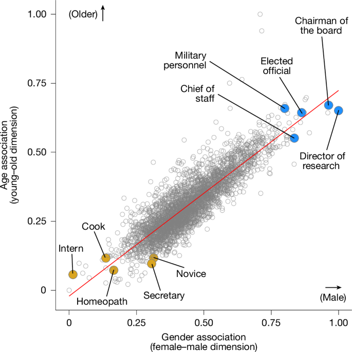
Correlation between age and gender associations for 3,495 social categories in GPT-2 Large. The horizontal axis presents the gender association from 0 (female) to 1 (male), and the vertical axis presents the age association from 0 (young) to 1 (old). The trend line shows the linear prediction according to an ordinary least squares regression. The orange highlighted categories illustrate some of the categories that have the youngest and most female associations, whereas the blue highlighted categories illustrate some of the categories that have the oldest and most male associations.

The systematic distortion of age–gender associations in online images, videos and text across popular platforms that we have identified raises concerns about how mainstream algorithms trained on these data might amplify the spread of this bias. We begin by examining possible algorithmic amplification in the visual modality to investigate whether exposure to visual content from the Google search engine amplifies age-related gender bias in people’s beliefs.

To answer this question, we report the results of a pre-registered experiment. We recruited a nationally representative sample of US participants from Prolific (n = 500), who were tasked with using Google to search for images of occupations related to science, technology and the arts (Extended Data Fig. 5; ‘Participant pool’ in Methods). In total, 459 participants completed the task. Each participant used Google to retrieve descriptions of 22 randomly selected occupations from a set of 54 (‘participant experience’ in Methods). The participants were randomized into treatment or control condition. In the treatment condition (hereafter ‘image condition’), the participants used Google Images to search for images of occupations, which they then uploaded to our survey. After uploading an image for an occupation, the participants were asked to label the gender of the image they uploaded and then to estimate the average age of someone in this occupation. The participants were also asked to rate their willingness to hire the person depicted in their uploaded image. In the control condition, the participants used Google Images to search for and upload images of basic unrelated categories (such as apple and guitar). After uploading a random image, the control participants were asked to estimate the average age of someone in a randomly selected occupation from the same set. The control participants were also asked to rate the ideal hiring age of someone in each occupation, as well as which gender (‘male’ or ‘female’) is most likely to belong to each occupation. This design allowed us to evaluate the treated participants’ age estimates of occupations after uploading an image of a man or woman compared with (1) the control participants’ age estimates formed without exposure to images of occupations and (2) the control participants’ age estimates conditional on their belief about which gender is most common in each occupation.

We began by testing the prediction that exposure to online images of occupations primes age-related gender bias in the participants’ beliefs. To test this prediction, we evaluated whether uploading an image of a woman (man) for each occupation is associated with a lower (higher) age estimate compared with the average age estimate of each occupation provided by those in the control condition who did not encounter online images of each occupation before providing their estimates. Figure 3a shows that the participants who uploaded an image of a woman estimated the average age of an occupation to be 5.46 years younger than those who uploaded an image of a man (t = −19.07; P = 2.2 × 10⁻¹⁶; Student’s t-test), holding occupation constant. Moreover, uploading an image of a woman led the participants to estimate a significantly lower age for each occupation (by 1.75 years) compared with the control participants (t = −11.32; P = 2.2 × 10⁻¹⁶), whereas uploading an image of a man led the participants to estimate a significantly higher age for each occupation (by 0.64 years) compared with those in the control condition (t = 3.42; P = 0.0006; Student’s two-tailed t-test).

Fig. 3: Googling for images of occupations amplifies age-based gender inequality in people’s beliefs.

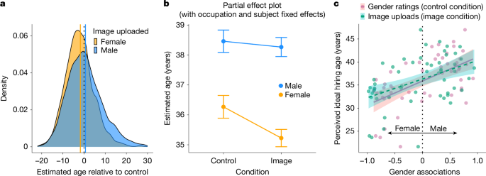
The participants (n = 459) from a nationally representative sample were randomized either to the ‘image’ condition, in which they googled for images of occupations (n = 54), or the ‘control’ condition, in which they googled for image-based descriptions of random categories (such as apple) unrelated to occupations. a, Average age of each occupation, as estimated by the participants in the image condition, broken down by whether they uploaded a female or male image of the occupation, centred relative to the average age of each occupation provided across all the participants in the control condition. b, Partial effect plot that controls for occupation and participant fixed effects while predicting the average age provided for each occupation depending on the gender of the image uploaded by the participants in the image condition or the gender the participants most associated with each occupation in the control condition. Data points display mean values, and error bars indicate 95% confidence intervals. c, Correlation between the gender association and perceived ideal hiring age of each occupation (averaged across all the participants in the control condition). The gender association of each occupation was measured separately according to the participants’ manual gender ratings in the control condition and the gender distribution of the images uploaded by the participants in the image condition. Data points show the average gender association and perceived ideal hiring age for each occupation according to each measure. Error bands show 95% confidence intervals.

Notably, these results hold when controlling for the participants’ gender and age, as well as whether their own demographics matched those of the people depicted in the images they uploaded (Supplementary Tables 19 and 20). Supplementary analyses further demonstrate that the participants’ estimates of the average ages of people in occupations are significantly correlated with the median age of these occupations according to the US census, indicating that the participants’ age judgements were coherent and consistent with ground truth sociodemographic distributions (Supplementary Tables 21 and 22).

Next, we leveraged the control condition to examine the effect of exposure to online images depicting occupations, above and beyond the participants’ existing biases about the gender composition of occupations. Specifically, we tested whether the participants in the treatment condition reported younger (older) ages when uploading images of women (men) for each occupation compared with the age estimates provided by the control participants, who reported believing that women (men) most often belonged to a given occupation. Figure 3b shows that the control participants who believed women are most likely to belong to a given occupation also estimated the average age of people in this occupation to be significantly younger (by 2.15 years), evidencing a baseline pattern of age-related gender bias in people’s judgements (β[male] = 2.15 years; standard error = 0.38; t = 5.55; P = 2.98 × 10⁻⁸). However, Fig. 3b further shows that this age gap is even higher among those in the treatment condition. The participants who uploaded an image of a woman for a given occupation reported estimating the age of people in this occupation to be significantly younger than the control participants who already believed that this occupation is female-skewed. This analysis controls for the specific occupation being evaluated, as well as the participants’ idiosyncratic judgements through occupation and participant fixed effects (β[gender × condition] = −0.84; standard error = 0.31; t = −2.69; P = 0.007). These results indicate that exposure to online images significantly exacerbates the perceived age gap between women and men, particularly by increasing the association between women and youth.

We conclude these experimental analyses by examining the practical consequences of this age-based gender bias by evaluating its impact on women’s and men’s perceived fit across occupations. Figure 3c shows that occupations that are more associated with women (men) are significantly correlated with the participants reporting lower (higher) recommended ages for whom to hire in this occupation. Figure 3c shows that the control participants’ perceived ideal age for hiring is strongly and positively correlated with the extent to which each occupation is associated with men, as measured by (1) the control participants’ manual gender ratings of occupations (r = 0.58; P = 3.52 × 10⁻⁶) and (2) the gender associations in the images uploaded by the participants in the image condition (r = 0.45; P = 0.0006; Pearson’s two-tailed correlation). These analyses provide evidence that age-related gender associations mediate people’s judgements of who is best to hire for a given occupation, with a preference towards hiring younger women and older men.

The above results are highly robust to whether (1) the participants provided gender ratings of occupations without estimating age (as captured by a separately replicated experiment⁶; Supplementary Fig. 17) and (2) the participants rated hireability using a Likert scale (Supplementary Fig. 18; see Supplementary Tables 23 and 24 for a full summary of all of our pre-registered hypotheses and the associated analyses and results). All of our main pre-registered hypotheses were strongly supported. Note that the framing of our study was updated in response to the review process, with no changes to the reporting of the experimental design or statistical results (see Supplementary Table 24 and the associated discussion for details).

Because popular artificial intelligence tools such as ChatGPT are trained on internet data, we further propose that ChatGPT will exhibit significant age-based gender bias in its textual representations and evaluations of occupations in professional resumes. Identifying age-related bias in ChatGPT would highlight a potential pathway through which this bias is widely propagated, given that more than 400 million people and two million businesses use ChatGPT weekly⁵⁷. By adapting prompt engineering techniques developed for auditing biases in ChatGPT’s resume generation⁵⁸, we prompted ChatGPT (v.GPT-4o mini) to create nearly 40,000 resumes for 54 occupations using 16 unique female and male names that were normalized to control for name popularity, familiarity, ethnicity and perceived age group, such that the male and female names were maximally similar along these dimensions (the same names were used in a recent auditing study⁵⁸) (see ‘Prompt design’ in Methods). This experiment consisted of two phases: resume generation and resume evaluation (Extended Data Fig. 6). All resumes were generated and evaluated in June 2024.

We began by examining the resume generation phase, in which we prompted ChatGPT to generate resumes across 54 occupations while varying the prompt across three conditions: (1) the control condition; (2) the control–gender condition; and (3) the treatment condition. In the control condition, we prompted ChatGPT to generate 50 resumes for each of the 54 occupations without specifying the name or gender of the applicant, resulting in 2,700 unique resumes. In the control–gender condition, we replicated the control condition, except that we also asked ChatGPT to include the gender of applicants in the resumes generated. Finally, in the treatment condition, we replicated the design of the control condition, except that our prompt included a specific name for the applicant and asked ChatGPT to generate a resume for the named applicant applying for the specified occupation (in this condition, ChatGPT was not asked to explicitly identify the gender of the named applicant). We used the same occupations in our image search experiment. In the treatment condition, we prompted ChatGPT 20 separate times for each name–gender–occupation prompt combination, yielding a total of 34,560 resumes and 17,280 resumes for each gender group. The resume features generated by ChatGPT were highly coherent and stable (Supplementary Fig. 19 and Supplementary Table 25).

Next, we evaluated the consequences that age-based gender biases in ChatGPT’s representations of resumes can have on its practical application as a hiring tool. We focused on one of ChatGPT’s most popular uses in the workplace: to evaluate, score and rank resumes to expedite hiring processes by focusing human recruiters on resumes with top scores⁵⁸. We prompted ChatGPT to evaluate each of the resumes generated in the first phase by providing a score between 1 and 100 to indicate the quality of each resume. All reported results are robust to altering the model temperature of ChatGPT (Supplementary Fig. 20).

We began by examining how altering the gender of a target applicant’s name affects the resumes that ChatGPT generates. We compared the resumes that ChatGPT generated in the treatment condition for female or male names while using a linear regression to control for the applicant name and occupation. As Fig. 4a indicates, when ChatGPT generated a resume for a female name, it generated resumes with significantly lower ages (by 1.6 years; t = 20.5; P = 7.09 × 10⁻⁹³), more recent graduation dates (by 1.3 years; t = 12.5; P = 1.18 × 10⁻³⁵) and fewer years of relevant experience (by 0.92 years; t = 5.39; P = 6.97 × 10⁻⁸) compared with male names (Student’s t-test; n = 34,560 resumes). Compared with the control condition, the resumes ChatGPT generated for female (male) applicants were significantly younger (older) and less (more) experienced than the resumes generated for the same occupations without any gender or name (all at the P < 0.00001 level; Student’s two-tailed t-test). Thus, ChatGPT exhibits age-based assumptions about women and men that are highly consistent with stereotypical associations relating to gendered ageism.

Fig. 4: Effect of gender and age on ChatGPT’s generation and evaluation of resumes.

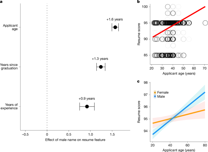
a, Partial effect plot in an ordinary least squares regression displaying the effect of a male applicant name (versus a female applicant name) on (1) applicant age; (2) years since the applicant’s graduation; and (3) the number of years of applicant’s relevant experience, while controlling for name and occupation. Only resumes from the treatment condition were examined in this analysis (n = 34,560), because this ensures that all resumes have either a male or female name and were produced through the same prompt. Error bars indicate 95% confidence intervals. b, Linear correlation between applicant age and ChatGPT’s rating of resume quality across all resumes (n = 39,560) from all conditions. Data points display the raw distribution of scores for each resume, with one data point per resume. The trend line reflects a standard bivariate linear trend. c, Partial effect plot displaying the interaction effect between applicant age and applicant gender on ChatGPT’s rating of resume quality, with fixed effects for applicant name, occupation and phase 1 condition (data from the control condition were excluded because of the lack of applicant gender; n = 37,060 resumes used in total). Error bands display 95% confidence intervals. ChatGPT’s temperature was set to its default value of 0.7.

These patterns of age-based gender bias in ChatGPT were replicated in the control–gender condition, in which ChatGPT generated its own name and gender classification for each occupation. When ChatGPT generated a male applicant for a given resume, this applicant was more likely to be older (by 1.3 years; t = 17.3; P = 2.2 × 10⁻¹⁶) and to have graduated less recently (by 1.2 years; t = 7.10; P = 2.29 × 10⁻¹²) than when it generated a resume for a female applicant, holding occupation constant (Student’s t-test; n = 2,500 resumes). Thus, the effects we observed were not dependent on the specific names used to prompt ChatGPT or on the overall prompt design in the treatment condition.

We next evaluated the consequences this bias had on how ChatGPT evaluated the quality of resumes. Across all occupations, Fig. 4b shows that ChatGPT’s judgements of resume quality were significantly and positively correlated with the age of the applicant that ChatGPT initially generated for the resume (r = 0.27; P = 2.2 × 10⁻¹⁶; t = 51.59; Pearson’s two-tailed correlation; n = 39,560 resumes). This result equally holds in a linear regression when we controlled for the occupation and name used to generate each application (β[age] = 0.04; t = 6.3; P = 2.96 × 10⁻¹⁰). Finally, we tested whether ChatGPT exhibits a preference not only for older applicants but also for older men specifically, consistent with the predictions of gendered ageism^6,7. We used linear regression to predict ChatGPT’s judgements of resume quality using an interaction between the age and gender of the applicant while holding occupation and applicant name constant. As shown in Fig. 4c, the model identified a highly significant and positive interaction between being male and older, indicating that the benefit of older age on ChatGPT’s judgements of resume quality is even greater if the applicant is male rather than female (β[male × age] = 0.04; t = 6.61; P = 3.66 × 10⁻¹¹). This interaction effect is robust to altering ChatGPT’s model temperature (Supplementary Fig. 20).

In this study, we have provided large-scale evidence that age-related gender bias pervades online media, including images, videos and texts across major platforms, and that the bias towards representing women as younger distorts ground truth realities on the actual ages of women and men throughout society. Our findings raise an alarm about the algorithmic amplification of age-related gender bias on the internet, especially considering that many mainstream machine learning algorithms are trained on these public datasets. Many of the image and text datasets examined in this study are used extensively as canonical training and benchmark datasets for developing artificial intelligence applications. Enormous harm can be caused by latent social biases that lurk in popular machine learning tools^59,60, and algorithmic bias typically arises from contaminated training data. Our study provides direct evidence that age-related gender bias is amplified by two of the most widely used algorithms today: the Google Image search engine and ChatGPT. Although companies such as Google and OpenAI invest heavily in reducing stereotypical content in their products⁶¹, most studies focus on single dimensions of bias, such as gender-based or race-based biases. Our study highlighted the critical need to account for multimodal and multidimensional forms of bias⁶², which are more challenging to detect but not less consequential in how people and algorithms represent the social world. The intersectional statistical bias we identified between gender and age may interact with other biases, such as relating to how women and men are depicted in terms of warmth and competence, revealing a promising direction for future research^63,64.

How might the digital distortion of age-related gender associations negatively affect women and men? Our results highlighted several key ways in which older women are likely to be disadvantaged by this bias. For example, when generating resumes, ChatGPT not only assumes that women are younger, but also that they have less overall experience. Consequently, ChatGPT is biased towards giving lower scores to resumes from younger women compared with older women while giving the highest scores to older men. Yet, ChatGPT also gives higher scores to resumes from young women than from young men, suggesting that young men may also be disadvantaged by this dual bias (Supplementary Fig. 18). However, a selection bias favouring younger women and older men may further reinforce gender inequalities at the systemic level, whereby women are preferentially hired into roles with lower status and authority but denied mobility, whereas older men continue to enjoy top positions. This resonates with our finding that online content is most likely to depict men as older than women for occupations with higher status and wealth.

A critical direction for future research is to investigate the causal mechanisms through which age-related gender bias seeps into and spreads through the images, videos and text of distinct platforms, each with its own unique audiences and distribution channels. Our results about objective differences in the ages of male and female celebrities visualized on IMDb, Wikipedia and Google probably reflect industry-specific mechanisms related to status dynamics, hiring biases and the objectification of women in entertainment media. Yet, these industry-specific drivers do not account for how strongly women and youth are semantically associated in massive bodies of online text from diverse sources, let alone in ChatGPT’s text-based representations and rankings of job candidates. A fascinating question for future work is to explore whether the aesthetic norms and hiring biases of entertainment media spill over into the distortion of age–gender associations throughout social life. A related question concerning supply-side factors concerns whether age-related gender bias in popular algorithms stems from inequalities in the gender of data contributors online. Studies suggest that Reddit users⁶⁵ and Wikipedia editors⁶⁶ are disproportionately male, and textual data from these platforms are frequently mined for training artificial intelligence models. Training artificial intelligence on datasets with greater gender equality in data contributors may provide an effective mitigation strategy.

This study highlights the increasingly prominent role of internet culture and algorithms in mediating our representation of the social world. As a recent review article emphasized⁶⁷, previous studies have been limited in their ability to concretely measure the diverse cultural meanings of age both in terms of its biological basis and its relevance to cultural notions of life stages (such as ‘youth’ and ‘childhood’). The strength of our approach is that it captures the cultural meanings of age and gender along many dimensions, from concrete time-stamped images to verbal descriptions of age categories across social roles and contexts. We revealed that the cultural meanings of gender and age are deeply linked on a massive scale across information modalities and in ways that reflect socioeconomic inequalities. Compelling evidence that these patterns are socially constructed comes from our finding that online associations between gender and age heavily distort the measurable ground truth reality of how people of different genders and ages are distributed throughout society. The extent to which algorithms entrench distortions of social reality en masse and to which this can be corrected is a vital topic for future research on internet policy and human cultural evolution. The methods we propose for measuring widespread stereotyped representations online and for grounding them in verifiable sociodemographic realities mark a crucial step in the fight against pervasive cultural inequalities, both online and beyond.

In this section, we detail the methods used in all parts of our analyses, including our observational comparisons of gender and age bias in online images, videos and texts, as well as our Google Image search experiment and our resume audit of ChatGPT. The pre-registration for our online image search experiment is available at https://osf.io/x9scm. This experiment was a successful replication of a previous study with a nearly identical design; the pre-registration of this previous study is available at https://osf.io/2b58d. This study was approved by the ethics review board at the University of California, Berkeley, where this study was conducted.

Observational methods

In what follows, we describe our observational methodology for collecting and analysing large bodies of images, videos and text online. With regard to the crowdsourcing methods applied to analysing our main Google and Wikipedia Image datasets, many of the methods described below (including the procedure and demographic details of the coder population) were reproduced from the original data collection summary provided as part of the first publication of these datasets⁶. In addition to this reproduced description, we include information on how age classifications of these images were collected, because this feature was not explored or discussed as part of the original publication of these datasets⁶.

Image data collection procedure

Our crowdsourcing methodology consisted of four steps. We began by identifying all social categories in WordNet⁶⁹, a canonical lexical database of English. WordNet captures 3,495 social categories, including occupations (such as doctor) and generic social roles (such as neighbour). We then gathered online images associated with each social category from Google and Wikipedia. Next, we applied the OpenCV deep learning module in Python to automatically extract the face from each image. Cropping faces helped us ensure that each face in each image was separately classified in a standardized manner while avoiding subjective biases in coders’ decisions for which face to focus on and categorize in each image. Finally, we hired 6,392 human coders from Amazon’s Mechanical Turk to manually classify the gender of the faces. Each face was classified by three unique annotators (as per established methodology^6,70,71), so that the gender of each face (‘male’ or ‘female’) could be identified on the basis of the majority (modal) gender classification across three coders. (We also gave coders the option of labelling the gender of faces as ‘non-binary’, but this option was only chosen in 2% of cases. Therefore, we excluded these data from our main analyses and recollected all classifications until each face was associated with three unique coders using either the male or female label.) Although coders were asked to label the gender of the faces presented, our measure was agnostic to which features the coders used to determine their gender classifications. They may have used facial features and features relating to the aesthetics of expressed gender, such as hair or accessories. In terms of age, each face was classified as belonging to one of the following age bins (the ordinal ranking of each bin is indicated in parentheses): (1) 0–11, (2) 12–17, (3) 18–24, (4) 25–34, (5) 35–54, (6) 55–74 and (7) 75+. Because the greater number of classification options for age led to fewer images associated with a majority-preferred age classification, we identified the age of each face by taking the average of the ordinal age bin judgements across the three coders. Each search was implemented from a fresh Google account with no previous history. Searches were run in August 2020 by ten distinct data servers in New York City. This study was approved by the institutional review board at the University of California, Berkeley, where this part of the study was conducted. All participants provided informed consent.

To collect images from Google, we followed a previous study by retrieving the top 100 images that appeared when using each of the 3,495 categories to search for images using the public Google Images search engine. (Google provides roughly 100 images for its initial search results.) Across the non-gendered and gendered searches, 3,489 categories could be associated with images containing faces in the Google Image search engine (specifically, 3,434 categories for the non-gendered searches and 2,960 for the gendered searches). To collect images from Wikipedia, we identified the images associated with each social category in the 2021 Wikipedia-based Image Text (WIT) Dataset⁷². WIT maps all images over Wikipedia to textual descriptions on the basis of the title, content and metadata of the active Wikipedia articles in which they appear. We were able to associate 1,251 social categories from WordNet with images in WIT (across all English articles) that supported stable classification as human faces with detectable ages, according to our coders. The coders identified 18% of images as not containing human faces, and these were removed from our analyses. We also asked all annotators to complete an attention check, which involved providing the correct answer to the common-sense question (What is the opposite of the word ‘down’?) using the following options: ‘fish’, ‘up’, ‘monk’ and ‘apple’. We removed the data from all annotators who failed an attention check (15%) and continued collecting classifications until each image was associated with the judgements of three unique coders, all of whom passed the attention check.

Demographics of human coders

The human coders were all US-based adults fluent in English. Supplementary Table 3 indicates that our main results are robust to controlling for the demographic composition of our human coders. Among our coders, 44.2% identified as being female, 50.6% as male, 3.2% as non-binary and the remaining preferred not to disclose. In terms of age (in years), 42.6% identified as 18–24, 22.9% as 25–34, 32.5% as 35–54, 1.6% as 55–74 and less than 1% as over 75. In terms of race, 46.8% identified as Caucasian, 11.6% as African American, 17% as Asian, 9% as Hispanic, 10.3% as Native American and the remaining as either mixed race or preferred not to disclose. In terms of political ideology, 37.2% identified as conservative, 33.8% as liberal, 20.3% as independent, 3.9% as other and the remaining preferred not to disclose. In terms of annual income, 14.3% reported making less than US$10,000, 33.4% reported US$10,000–50,000, 22.7% reported US$50,000–75,000, 14.9% reported US$75,000–100,000, 10.5% reported US$100,000–150,000, 2.8% reported US$150,000–250,000, less than 1% reported more than US$250,000 and the remaining preferred not to disclose. In terms of the highest level of education acquired by the annotator, 2.7% selected ‘below high school’, 17.5% selected ‘high school’, 29.2% selected ‘technical/community college’, 34.5% selected ‘undergraduate degree’, 14.8% selected ‘master’s degree’, less than 1% selected ‘doctorate degree’ and the remaining preferred not to disclose.

Image and video datasets

To measure age-related gender bias in online images and videos, we analysed a range of open-source datasets collected either for social science research or for training face recognition algorithms, none of which examined or reported correlations between the gender and age of the people depicted. In total, we examined more than one million images from five main online sources: Google, Wikipedia, IMDb, Flickr and YouTube, as well as the Common Crawl (created by randomly scraping content from across the world-wide web), each with distinct ways of sourcing and aggregating data. We measured gender and age using a variety of techniques, including human judgements, machine learning and ground truth data on the self-reported gender and true time-stamped age of the people depicted. Our statistical analyses did not control for multiple comparisons because all tests were theoretically guided and did not involve an agnostic permutation over a set of pairwise comparisons. Although we examined many datasets, our main analyses examined a single correlation (between gender and age) within each dataset separately. We now describe each of these datasets.

First, we used large-scale crowdsourcing to identify age-related gender bias in a new dataset of images from Google and Wikipedia (which was originally collected for a recently published study that did not examine age-related classifications)⁶. This dataset⁶ contains the top 100 Google images associated with each of the 3,435 social categories contained within WordNet⁶⁹, a lexical ontology that maps the taxonomic structure of the English language. These categories include occupations (such as ‘physicist’) and generic social roles (such as ‘colleague’). For each category, this dataset contains the top 100 images that appear in Google Images when searching for (1) the category on its own (such as ‘doctor’); (2) the female version of the category (such as ‘female doctor’); and (3) the male version of the category (such as ‘male doctor’). The gendered searches were completed only for the 2,960 non-gendered categories (for example, the searches did not include ‘male aunt’). Altogether, this yielded 657,035 unique images containing faces from Google. Searches were run from ten distinct data servers in New York City. Because Google is known to customize search results on the basis of the location from which the search is run⁷², we show that our results are robust to replicating this data collection pipeline while collecting Google Images from six distinct cities around the world (Supplementary Fig. 3).

This dataset also leveraged human coders to classify the age and gender of faces in Wikipedia images associated with as many WordNet social categories as possible in the 2021 WIT Dataset⁶⁸. WIT maps all images over Wikipedia to textual descriptions on the basis of the title, content and metadata of the active Wikipedia articles in which they appear. WIT includes images of 1,251 social categories from WordNet across all English Wikipedia articles, in total yielding 14,709 faces.

We hired 6,392 human annotators from Amazon’s Mechanical Turk to classify the gender and age of the faces in these images. Each face was classified by three unique annotators^6,70,71 so that the gender of each face (male or female) could be identified on the basis of the majority gender classification across three coders. (We also gave coders the option of identifying the gender of faces as non-binary, but this option was chosen in less than 2% of cases. Therefore, we excluded these data from our main analyses.) In terms of age, each face was classified as belonging to one of the following age bins (in years): (1) 0–11, (2) 12–17, (3) 18–24, (4) 25–34, (5) 35–54, (6) 55–74 and (7) 75+. Because the greater number of classification options for age led to fewer images with a majority-preferred classification, we identified the age of each face by taking the average of the ordinal age bin judgements across the three coders (our main results hold when using the modal age judgement; Supplementary Fig. 4). Our findings continued to hold when controlling for annotator demographics and intercoder agreement, which was high in our sample (Supplementary Fig. 5 and Supplementary Table 3). We also conducted a separate validation task, in which the true gender and age of the faces being classified were known. The results indicate that our coders exhibited reliable and accurate gender and age judgements, with no biases as a function of gender (Supplementary Tables 4 and 5). Sensitivity tests further showed that even if our coders were hypothetically biased in their ability to estimate age as a function of gender, this would not disrupt the statistical significance or directionality of our findings (Supplementary Fig. 6).

We extended our findings by examining age-related gender bias in two large corpora of online images collected from three main websites (IMDb, Wikipedia and Google) for which the self-identified gender and true age of the faces were objectively inferred. This extension allowed us to examine whether women are objectively younger than men in online images, without depending on age predictions from human coders or machine learning algorithms. The first corpus was the 2018 IMDb–Wiki dataset⁴³, which consisted of more than half a million images of celebrities from IMDb and Wikipedia on the basis of those depicted in the top 100,000 most visited IMDb pages. Each image in this dataset was time-stamped for when the photograph was taken, allowing the age of each face to be inferred on the basis of the celebrity’s date of birth, which is publicly available through their open profile on IMDb and Wikipedia. This dataset yielded 451,570 images from IMDb and 57,932 images from Wikipedia. The second corpus was the 2014 CACD⁴⁴, which consisted of 163,446 images collected from the Google Image search engine depicting 2,000 celebrities, comprising the top 50 most popular celebrities each year from 1951 to 1990. The creators of CACD collected time-stamped images by using Google Image search to retrieve images associated with each celebrity from 2004 to 2013 (for example, by searching ‘Emma Watson 2004’ through ‘Emma Watson 2013’). We merged the CACD and IMDb–Wiki dataset⁴³ to identify the gender of 1,825 celebrities in the CACD (50% are female celebrities). All images from both datasets containing ages below 0 and above 100 were removed to maximize data quality. Each dataset identified the exact age of the celebrities at the time they were depicted in each photograph by determining the date of birth and gender of each celebrity on their public IMDb and Wikipedia pages and then by comparing this information to the time-stamped date of when each photograph was taken.

Finally, we examined images from four publicly available training datasets widely used to train automated face recognition algorithms. In these canonical datasets, the gender and age classifications were on the basis of a combination of automated machine learning classifications and verification through human annotation. This includes the 2017 UTK dataset⁴⁶ consisting of 20,000 images scraped randomly from across the world-wide web using search engines and public repositories, the 2014 Adience dataset⁴⁷ consisting of 26,580 images randomly sampled from Flickr, a public image-based social media platform, and the 2008 LFW⁴⁸ dataset consisting of 13,233 images randomly scraped from online news websites. Finally, we examined images of faces extracted from screenshots of YouTube videos using two datasets. The first was the 2011 YouTube Faces dataset⁵⁰ consisting of 3,425 YouTube videos and 3,645 images of celebrities. The second one was the 2022 CelebV-HQ⁵¹ dataset consisting of 35,666 images formed by identifying public lists of celebrities on Wikipedia and automatically collecting the top 10 YouTube videos associated with each celebrity.

Comparing online images with the census

We were able to match 867 social categories from our main Google image (Fig. 1a) dataset to occupational categories in the US census. The US Bureau of Labor Statistics recently released a breakdown of the median age of each gender, from 2019 to 2023, across five industries: sales, services, natural resources and construction, production and transportation and management. The census assigns each occupation to one of these industries, allowing those occupations matched in our Google image dataset to be assigned a census industry. We estimated the relationship between gender and age at the industry level by averaging the age associations in Google Images across all occupations within a given industry (averaged within each occupation and then across occupations at the industry level). The census age groupings are highly similar to the age groupings the coders used when judging faces. Supplementary Tables 8 and 9 present the robustness of our results to a range of statistical controls.

Collecting judgements of occupational status

We collected a nationally representative sample of 1,002 US-based participants who provided their subject evaluations of the status and prestige of occupations. Each participant evaluated 20 randomly sampled occupations from a broader set of 867 WordNet social categories that could be matched with corresponding occupations in the US census. Through randomization, each category was evaluated by 27 unique participants on average (minimum of 15 participants). For each occupation, the participants rated (1) its status using the following scale (How would you rate the social status of someone belonging to this occupation? −2, very negative; −1, negative; 0, neutral; 1, positive; 2, very positive) and (2) its prestige using the following scale (To what extent do you agree that it is prestigious to belong to this occupation? −2, strongly disagree; −1, disagree; 0, neutral; 1, agree; 2, strongly agree). We also asked the participants to rate the status/prestige through the standard question from the general social survey, which asked them to place occupations on a ladder containing 10 rungs, where the bottom rung indicates occupations with very low status, income, education and prestige, whereas the highest rung indicates occupations with very high status, income, education and prestige (Supplementary Fig. 11). The participants’ answers across all three questions were highly correlated (all paired Pearson’s correlations above 0.85; Supplementary Fig. 9). In our main results shown in Extended Data Fig. 4, we first averaged all participants’ judgements of each occupation across the (1) status and (2) prestige question and then assigned each occupation a single status score by taking the mean of its average status and prestige score. In the Supplementary Information, we show that all of our results hold when examining each question separately and when examining the participants’ judgements using the standard social status question from the General Social Survey (GSS) (Supplementary Fig. 11 and Supplementary Tables 10–13). Note that Prolific’s nationally representative sample of the US population size allows for a maximum of 800 participants. However, this sample size was not large enough to gain sufficiently powered judgements across all 867 occupational categories; therefore, an extra sample of US participants was recruited until all occupations reached a minimum of 15 evaluations from independent participants. All results are robust to a range of statistical controls (Supplementary Tables 10–13).

Measuring age and gender in online text

To measure age-related gender bias in large bodies of internet text, we leveraged word embedding models trained on massive amount of internet data. These models were designed to construct a high-dimensional vector space on the basis of the co-occurrence of words (for example, whether two words appear in the same sentence), such that words with similar meanings are closer in this vector space. Technically, these embedding spaces also capture higher-order similarities on the basis of whether words co-occur in similar linguistic contexts (that is, in association with related sets of words), without requiring words to directly appear together. We harnessed recent advances in natural language processing to extract demographic dimensions in word embedding models that capture the extent to which existing demographics underlie the cultural connotations of categories. We identified both gender and age dimensions. We briefly describe this methodology below.

Word embedding models leverage the frequency of word co-occurrences in text to position words in an n-dimensional space such that words that frequently co-occur together are more closely located in this n-dimensional space. The ‘embedding’ for a given word identifies the specific position of this word in this n-dimensional space. The cosine distance between word embeddings in this n-dimensional space provides a robust measure of semantic similarity that captures the similarity of the semantic contexts in which words appear⁶. To extract a gender dimension in word embedding space, we harnessed the ‘geometry of culture’ method of Kozlowski et al.⁷³. This method was originally developed for static embedding models such as Word2Vec and GloVe; therefore, we incorporated key adjustments that enable its application to contextualized embeddings through generative transformer models such as GPT-2 Large. We identified two clustered regions in the word embedding space corresponding to conventional representations of females and males. Specifically, the female cluster consisted of ‘woman’, ‘her’, ‘she’, ‘female’ and ‘girl’, whereas the male cluster consisted of ‘man’, ‘his’, ‘he’, ‘male’ and ‘boy’. For each social category in WordNet, we calculated the average cosine distance between this category and both the female and male clusters. Each category was associated with two numbers: its cosine distance with the female cluster (averaged across its cosine distance with each term in the female cluster) and its cosine distance with the male cluster (averaged across its cosine distance with each term in the male centroid). Taking the difference between the cosine distance of a category with the female and male centroids allowed each category to be positioned along a −1 (female) to 1 (male) scale in the embedding space. Although we recognize that gender is fundamentally non-binary, we built upon a previous study that leveraged this binary framework⁷³ to identify biases in the extent to which people associate concepts with men or women.

The issue with applying this approach to contextualized embeddings is that the embedding associated with an individual word can be sharply different from the embedding associated with this word within a larger context, for example, within a surrounding sentence. For this reason, we modified the geometry of culture method by creating male and female poles consisting of many parallel sentences that vary only in whether they mention the corresponding male or female version of a pronoun. For example, the male pole consists of sentences such as ‘he is a boy’ and ‘his hobbies are very masculine’, whereas the analogues of these sentences in the female pole are ‘she is a girl’ and ‘her hobbies are very feminine’. Fifty sentences were used to form each pole. All sentences used are provided in Supplementary Tables 14 and 15. We conducted key robustness tests to verify the validity of our methods and the robustness of our results to the use of different sentences along the gender pole (Supplementary Fig. 13). In our supplementary analyses involving static embedding models, we used the original geometry of culture approach.

We used this same approach to construct an age dimension in word embedding models. For static embedding models, we identified two clustered regions in the word embedding space corresponding to younger and older ages. Specifically, the younger cluster consisted of the words ‘child’, ‘teenager’ and ‘adolescent’, whereas the older cluster consisted of the words ‘adult’, ‘senior’ and ‘elder’. All results are highly robust to increasing the number of words used to construct this age dimension. For example, our results replicate when defining the younger cluster using the words ‘young’, ‘youth’, ‘childhood’, ‘child’, ‘baby’, ‘infant’, ‘teen’, ‘teenager’ and ‘adolescent’, as well as when defining the older cluster using the words ‘old’, ‘elder’, ‘elderly’, ‘adulthood’, ‘adult’, ‘senior’, ‘parent’, ‘retired’ and ‘aged’. We used the same technique to sort categories along a −1 (young) to 1 (old) scale in the embedding space. Similarly, to examine age associations in contextualized embedding models, we generated 50 sentences that hold everything constant while varying whether the age term involved indicates a young or old age (see Supplementary Table 15 for a full list of the age sentences used to create the contextualized age pole).

In all cases examining static models, to compute the distances between the vectors of social categories represented by bigrams (such as ‘professional dancer’), we used the Phrases class in the gensim Python package, which provided a pre-built function for identifying and calculating distances for bigram embeddings. This method works by identifying an n-dimensional vector of middle positions between the vectors corresponding separately to each word in the bigram (for example, ‘professional’ and ‘dancer’). This technique then treats the middle vector as the singular vector corresponding to the bigram ‘professional dancer’ and is thereby used to calculate the distances from other category vectors. This method is not necessary in contextual language models, which provide unique embeddings for n-grams as distinct from their component words.

Once the corresponding demographic dimensions were constructed for each model, we evaluated the correlation between gender and age associations across 3,495 social categories from WordNet (the same categories examined in our image analyses above). To simplify the presentation of how this gender and age dimensions are correlated, we used min-max normalization to convert the gender dimension into a 0 (female) to 1 (male) association, which, in effect, represents the extent to which each category carries male associations relative to all other categories. We applied the same approach to produce a normalized 0 (young) to 1 (old) dimension, which captures the extent to which each category is associated with older ages relative to all other categories. The supplementary analyses showed that our results are highly robust to varying our technique for constructing the age and gender dimensions (Supplementary Fig. 13 and Supplementary Tables 14 and 15).

In the main text, we present our results while analysing the largest open-source large language model from OpenAI (GPT-2 Large⁵⁶), for which word embeddings can be robustly and transparently extracted and examined. GPT-2 Large is one of the largest and most popular open-source language models, trained on billions of words from the 2019 WebText dataset, which primarily comprises Reddit data and the diverse web content (including articles and books) to which these Reddit data are linked. In the supplementary analyses, we showed that these results replicate when examining a wide range of models, including Word2Vec, GloVe, BERT, FastText, RoBERTa and GPT-4, all of which vary in their dimensionality and data sources, as well as the year in which their training data were collected, ranging from 2013 to 2023. We focus our main results on GPT-2 Large, not only because of its scale and popularity, but also because its open-source nature allows us to transparently access and analyse its word embeddings. GPT-4, by contrast, is a closed-source model that relies on using OpenAI’s private application programming interface, which limits the interpretability of our method. Nevertheless, supplementary analyses showed that our results replicate when examining this closed-source model (Supplementary Figs. 14 and 15).

Experimental methods with human participants

Participant pool

We invited a nationally representative sample of participants (n = 500) from Prolific. Prolific is a popular online panel for social science research that provides prescreening functionality specifically for recruiting a nationally representative sample of the USA along the dimensions of sex, age and ethnicity. The participants were invited to partake in the study only if they were based in the USA, were fluent English speakers and were over 18 years old. A total of 52% of participants were female (no participants identified as non-binary). The average age of participants was 45.2 (45.9 for women; 44.6 for men). Our sample size was selected to emulate the sample size of a recent experiment with a highly similar design, which effectively measured statistically powered outcomes⁶. There was an attrition rate of 9.2% of participants (which is within the common range of attrition for online experiments), such that 459 participants completed the task. Our results only examined data from the participants who completed the experiment to ensure data quality. All the participants provided informed consent before participating. This experiment was run on 10 November 2023.

Participant experience

Extended Data Fig. 4 presents a schematic of the full experimental design. This experiment was approved by the Institutional Review Board at the University of California, Berkeley. In this experiment, the participants were randomized to one of two conditions: (1) the image condition (in which they used the Google Image search engine to retrieve images of occupations) and (2) the control condition (in which they used the Google Image search engine to retrieve images of random, non-gendered categories, such as ‘apple’). In the image condition, after uploading an image for a given occupation, the participants were asked to label the gender of the image they uploaded and then to estimate the average age of someone in this occupation. The participants in the image condition were also asked to rate their willingness to hire the person depicted in their uploaded image (Supplementary Fig. 18). After uploading a given random image, the control participants were then asked to estimate the average age of someone in a randomly selected occupation from the same set. The control participants were also asked to rate the ideal hiring age of someone in each occupation, as well as which gender (male or female) was most likely to belong to each occupation. This design allowed us to evaluate the treated participants’ age estimates after uploading an image of a man or woman compared with (1) the control participants’ age estimates that were formed without exposure to images of occupations and (2) the control participants’ age estimates conditional on which gender they think is most common in each occupation. All participants regardless of condition completed this sequence for 22 occupations (randomly sampled from a set of 54 occupations held constant across conditions). On average, the participants took 35 min to complete the task. All participants were compensated at the rate of US$15 per hour for their time.

The occupations that the participants identified were selected to include professions from science, technology, engineering and mathematics and the liberal arts. We used the exact list of occupations leveraged in a recent experiment of a similar design (focusing only on gender, not age) to compare results and evaluate replicability⁶. Here is the full pre-registered set: immunologist, mathematician, harpist, painter, piano player, aeronautical engineer, applied scientist, geneticist, astrophysicist, professional dancer, fashion model, graphic designer, hygienist, educator, intelligence analyst, logician, intelligence agent, financial analyst, chief executive officer, clarinetist, chiropractor, computer expert, intellectual, climatologist, systems analyst, programmer, poet, astronaut, professor, automotive engineer, cardiologist, neurobiologist, English professor, number theorist, marine engineer, bookkeeper, dietician, model, trained nurse, cosmetic surgeon, fashion designer, nurse practitioner, art teacher, singer, interior decorator, media consultant, art student, dressmaker, English teacher, literary agent, social worker, screen actor, editor-in-chief and schoolteacher.

Experimental methods with ChatGPT

Prompt design

The control condition in the resume generation phase used the following prompt (adapted from a recent audit study⁵⁸): ‘Write a detailed and concise resume for someone applying for a position in the role of [occupation] in the United States. Include the following sections: date of birth in month/day/year format, education with graduate date in month/day/year format, total number of years of relevant experience in numeric format and a numbered list of relevant skills’. This prompt differs from that of a previous study by prompting ChatGPT to include the applicants’ age and years of experience. We prompted ChatGPT 50 separate times for each occupation, resulting in 2,700 unique resumes in the control condition.

The control–gender condition in the resume generation phase replicated the design of the control condition, except it also asked ChatGPT to include each applicant’s gender in the resumes generated across the 54 occupations. This led to the following updated prompt: ‘Write a detailed and concise resume for someone applying for a position in the role of [occupation] in the United States. Include the following sections: gender of the applicant (male or female), date of birth in month/day/year format, education with graduate date in month/day/year format, total number of years of relevant experience in numeric format and a numbered list of relevant skills’. We prompted ChatGPT 50 separate times for each gender–occupation prompt combination, yielding 2,700 unique resumes in this condition.

The treatment condition in the resume generation phase replicated the design of the control condition, except that its prompt included a specific name for the applicant and asked ChatGPT to generate a resume for this named applicant applying for the specified occupation. We used 16 female names and 16 male names, all normalized in terms of popularity, familiarity, ethnicity and perceived age group, such that the male and female names were maximally similar along these dimensions. These names were developed and deployed by Armstrong et al.⁵⁸ for a related auditing task that did not involve requesting explicit age information to examine age-related gender bias. The female and male names validated by Armstrong et al.⁵⁸ included four names for the following ethnic identities: Hispanic, Asian, white people and Black people (four names per gender per ethnicity yielded 16 names for each gender). The prompt in this condition read: ‘[name] is applying for a position in the role of [occupation] in the United States. Write a detailed and concise resume for [name]. Include the following sections: date of birth in month/day/year format, education with graduate date in month/day/year format, total number of years of relevant experience in numeric format and a numbered list of relevant skills’. We prompted ChatGPT with this request 20 separate times for each name–gender–occupation prompt combination, yielding 34,560 resumes in total and 17,280 resumes for each gender group. This excludes the rare cases where ChatGPT failed to produce a resume (for example, by generating an empty JavaScript Object Notation structure without any resume-related information).

In the resume evaluation phase, we prompted ChatGPT to evaluate each resume from the resume generation phase by providing a score between 1 and 100 to indicate the quality of each resume. Specifically, we deployed the following prompt (adapted from Armstrong et al.⁵⁸): ‘Given the following job title and resume, rate the resume with a score between 1 and 100 to capture the quality of the resume and its fit with the job title. 1 is a low score, while 100 is a high score. Only return a score’.

Reporting summary

Further information on research design is available in the Nature Portfolio Reporting Summary linked to this article.

All data associated with this study can be downloaded from GitHub at https://github.com/drguilbe/distortion_age_gender_online/. The pre-registration for our experiment is available at https://osf.io/x9scm.

All codes associated with this study can be downloaded from GitHub at https://github.com/drguilbe/distortion_age_gender_online/.

References

Authors and Affiliations

1. Graduate School of Business, Stanford University, Stanford, CA, USA

   Douglas Guilbeault

2. Haas School of Business, University of California, Berkeley, Berkeley, CA, USA

   Solène Delecourt

3. Autonomy Institute, London, UK

   Bhargav Srinivasa Desikan

4. Oxford Internet Institute, University of Oxford, Oxford, UK

   Bhargav Srinivasa Desikan

Contributions

D.G. and S.D. designed the project. D.G. analysed the data. D.G. and B.S.D. developed the algorithmic methods and collected the data. D.G. wrote the paper. S.D. and B.S.D. assisted with editing the paper.

Corresponding author

Correspondence to Douglas Guilbeault.

Competing interests

The authors declare no competing interests.

Peer review information

Nature thanks April H. Bailey and the other, anonymous, reviewer(s) for their contribution to the peer review of this work. Peer reviewer reports are available.

Open Access This article is licensed under a Creative Commons Attribution-NonCommercial-NoDerivatives 4.0 International License, which permits any non-commercial use, sharing, distribution and reproduction in any medium or format, as long as you give appropriate credit to the original author(s) and the source, provide a link to the Creative Commons licence, and indicate if you modified the licensed material. You do not have permission under this licence to share adapted material derived from this article or parts of it. The images or other third party material in this article are included in the article’s Creative Commons licence, unless indicated otherwise in a credit line to the material. If material is not included in the article’s Creative Commons licence and your intended use is not permitted by statutory regulation or exceeds the permitted use, you will need to obtain permission directly from the copyright holder. To view a copy of this licence, visit http://creativecommons.org/licenses/by-nc-nd/4.0/.

Reprints and permissions

References

Madon, S., Guyll, M., Hilbert, S. J., Kyriakatos, E. & Vogel, D. L. Stereotyping the stereotypic: when individuals match social stereotypes. J. Appl. Social Psychol. 36, 178–205 (2006).
Jussim, L. et al. in Handbook of Prejudice, Stereotyping, and Discrimination 2nd edn (ed. Nelson, T. D.) 31–63 (Psychology Press, 2015).
Jussim, L., Crawford, J. T. & Rubinstein, R. S. Stereotype (In)accuracy in perceptions of groups and individuals. Curr. Dir. Psychol. Sci. 24, 490–497 (2015).
Puddifoot, K. How Stereotypes Deceive Us (Oxford Univ. Press, 2021).
Bai, X., Fiske, S. T. & Griffiths, T. L. Globally inaccurate stereotypes can result from locally adaptive exploration. Psychol. Sci. 33, 671–684 (2022).
Guilbeault, D. et al. Online images amplify gender bias. Nature 626, 1049–1055 (2024).
Itzin, C. & Phillipson, C. in Gender, Culture and Organizational Change (eds Itzen, C. & Newman, J.) 84–95 (Routledge, 1995).
Older Women: Inequality at the Intersection of Age and Gender https://data.unwomen.org/publications/older-women-inequality-intersection-age-and-gender (United Nations, 2022).
Diehl, A., Dzubinski, L. M. & Stephenson, A. L. Women in leadership face ageism at every age. Harvard Business Review https://hbr.org/2023/06/women-in-leadership-face-ageism-at-every-age (2023).
Allport, G. W. The Nature of Prejudice (Addison-Wesley, 1954).
Tajfel, H. in Intergroup Relations: Essential Readings (eds Hogg, M. A. & Abrams, D.) 132–145 (Psychology Press, 2001).
Fiske, S. T. & Tablante, C. B. in APA Handbook of Personality and Social Psychology, Volume 1: Attitudes and Social Cognition (eds Mikulincer, M. et al.) 457–507 (American Psychological Association, 2015).
Bartholomew, D. J. Measuring Intelligence: Facts and Fallacies (Cambridge Univ. Press, 2004).
Nosek, B. A. et al. National differences in gender–science stereotypes predict national sex differences in science and math achievement. Proc. Natl Acad. Sci. USA 106, 10593–10597 (2009).
Global Report on Ageism www.who.int/publications-detail-redirect/9789240016866 (Demographic Change and Healthy Ageing & World Health Organization, 2021).
Gender pay gap widens as women age: women consistently earn less than men. United States Census Bureau www.census.gov/library/stories/2022/01/gender-pay-gap-widens-as-women-age.html (2022).
Cecco, L. Anger as Lisa LaFlamme dropped as Canada TV anchor after going grey. The Guardian https://webstories.theguardian.com/stories/uk/2022/aug/22/anger-as-lisa-laflamme-dropped-as-canada-tv-anchor-after-going-grey/ (2022).
Spedale, S., Coupland, C. & Tempest, S. Gendered ageism and organizational routines at work: the case of day-parting in television broadcasting. Organ. Stud. 35, 1585–1604 (2014).
Duncan, C. & Loretto, W. Never the right age? Gender and age-based discrimination in employment. Gender Work Organ. 11, 95–115 (2004).
Ramati-Ziber, L., Shnabel, N. & Glick, P. The beauty myth: prescriptive beauty norms for women reflect hierarchy-enhancing motivations leading to discriminatory employment practices. J. Pers. Soc. Psychol. 119, 317–343 (2020).
MacArthur, H. J., Cundiff, J. L. & Mehl, M. R. Estimating the prevalence of gender-biased language in undergraduates’ everyday speech. Sex Roles 82, 81–93 (2020).
Miller, K. L. I’m a manager, but to my boss and colleagues, I’m a ‘girl’. Washington Post www.washingtonpost.com/business/economy/im-a-manager-but-to-my-boss-and-colleagues-im-a-girl/2019/05/10/d18fb3ea-71d0-11e9-9eb4-0828f5389013_story.html (2019).
Ridgeway, C. L. in Framed by Gender: How Gender Inequality Persists in the Modern World (ed. Ridgeway, C. L.) 32–55 (Oxford Univ. Press, 2011).
Martin, A. E., Guevara Beltran, D., Koster, J. & Tracy, J. L. Is gender primacy universal? Proc. Natl Acad. Sci. USA 121, e2401919121 (2024).
Shmerling, R. Why men often die earlier than women. Harvard Health www.health.harvard.edu/blog/why-men-often-die-earlier-than-women-201602199137 (2016).
Ducharme, J. Why U.S. women now live 6 years longer than men. Time Magazine https://time.com/6334873/u-s-life-expectancy-gender-gap/ (2023).
Chatman, J. A., Sharps, D., Mishra, S., Kray, L. J. & North, M. S. Agentic but not warm: age-gender interactions and the consequences of stereotype incongruity perceptions for middle-aged professional women. Organ. Behav. Hum. Decis. Processes 173, 104190 (2022).
Martin, A. E., North, M. S. & Phillips, K. W. Intersectional escape: older women elude agentic prescriptions more than older men. Pers. Soc. Psychol. Bull. 45, 342–359 (2019).
Garg, N., Schiebinger, L., Jurafsky, D. & Zou, J. Word embeddings quantify 100 years of gender and ethnic stereotypes. Proc. Natl Acad. Sci. USA 115, E3635–E3644 (2018).
Jones, J. J., Amin, M. R., Kim, J. & Skiena, S. Stereotypical gender associations in language have decreased over time. Sociol. Sci. 7, 1–35 (2020).
Williams, W. M. & Ceci, S. J. National hiring experiments reveal 2:1 faculty preference for women on STEM tenure track. Proc. Natl Acad. Sci. USA 112, 5360–5365 (2015).
Chan, J. & Wang, J. Hiring preferences in online labor markets: evidence of a female hiring bias. Manage. Sci. 64, 2973–2994 (2018).
Fiske, S. T. Prejudices in Cultural Contexts: Shared stereotypes (gender, age) versus variable stereotypes (race, ethnicity, religion). Perspect. Psychol. Sci. 12, 791–799 (2017).
Handy, J. & Davy, D. Gendered ageism: older women’s experiences of employment agency practices. Asia Pac. J. Hum. Resour. 45, 85–99 (2007).
Messner, M. A., Duncan, M. C. & Jensen, K. Separating the men from the girls: the gendered language of televised sports. Gend. Soc. 7, 121–137 (1993).
Lincoln, A. E. & Allen, M. P. Double jeopardy in Hollywood: age and gender in the careers of film actors, 1926–1999. Sociol. Forum 19, 611–631 (2004).
Hoegele, D., Schmidt, S. L. & Torgler, B. The importance of key celebrity characteristics for customer segmentation by age and gender: does beauty matter in professional football? Rev. Manag. Sci. 10, 601–627 (2016).
Edström, M. Visibility patterns of gendered ageism in the media buzz: a study of the representation of gender and age over three decades. Fem. Media Stud. 18, 77–93 (2018).
Martin, D. et al. The spontaneous formation of stereotypes via cumulative cultural evolution. Psychol. Sci. 25, 1777–1786 (2014).
Guilbeault, D., Baronchelli, A. & Centola, D. Experimental evidence for scale-induced category convergence across populations. Nat. Commun. 12, 327 (2021).
Mastroianni, A. M. & Gilbert, D. T. The illusion of moral decline. Nature 618, 782–789 (2023).
Bailey, A. H., Williams, A. & Cimpian, A. Based on billions of words on the internet, people = men. Sci. Adv. 8, eabm2463 (2022).
Rothe, R., Timofte, R. & Van Gool, L. Deep expectation of real and apparent age from a single image without facial landmarks. Int. J. Comput. Vis. 126, 144–157 (2018).
Chen, B.-C., Chen, C.-S. & Hsu, W. H. in Computer Vision – ECCV 2014 (eds Fleet, D. et al.) 768–783 (Springer, 2014).
Porter, C. & Serra, D. Gender differences in the choice of major: the importance of female role models. Am. Econ. J. Appl. Econ. 12, 226–254 (2020).
Zhang, Z., Song, Y. & Qi, H. Age progression/regression by conditional adversarial autoencoder. In Proc. IEEE Conference on Computer Vision and Pattern Recognition (CVPR) 4352–4360 (IEEE Computer Society, 2017).
Eidinger, E., Enbar, R. & Hassner, T. Age and gender estimation of unfiltered faces. IEEE Trans. Inf. Forensics Secur. 9, 2170–2179 (2014).
Huang, G. B., Ramesh, M., Berg, T. & Learned-Miller, E. Labeled Faces in the Wild: A Database for Studying Face Recognition in Unconstrained Environments https://inria.hal.science/inria-00321923v1/preview/Huang_long_eccv2008-lfw.pdf#page=2 (University of Massachusetts and Stony Brook University, 2008).
McGrady, R., Zheng, K., Curran, R., Baumgartner, J. & Zuckerman, E. Dialing for videos: a random sample of YouTube. J. Quant. Descr. Digital Media 3, 1–85 (2023).
Wolf, L., Hassner, T. & Maoz, I. Face recognition in unconstrained videos with matched background similarity. In Proc. CVPR 2011 529–534 (IEEE, 2011).
Zhu, H. et al. CelebV-HQ: a large-scale video facial attributes dataset. In Computer Vision – ECCV 2022 (eds Bertino, E. et al.) 650–667 (Springer, 2022).
Ridgeway, C. L. & Diekema, D. in Gender, Interaction, and Inequality (ed. Ridgeway, C. L.) 157–180 (Springer, 1992).
Ridgeway, C. L. Why status matters for inequality. Am. Sociol. Rev. 79, 1–16 (2014).
Occupational prestige ratings. GitHub https://occupational-prestige.github.io/opratings/index.html.
Kochhar, R. The enduring grip of the gender pay gap. Pew Research Center www.pewresearch.org/social-trends/2023/03/01/the-enduring-grip-of-the-gender-pay-gap/ (2023).
Radford, A. et al. Language models are unsupervised multitask learners. OpenAI Blog 1 https://cdn.openai.com/better-language-models/language_models_are_unsupervised_multitask_learners.pdf (2019).
Kant, R. OpenAI’s weekly active users surpass 400 million. Reuters www.reuters.com/technology/artificial-intelligence/openais-weekly-active-users-surpass-400-million-2025-02-20/ (2025).
Armstrong, L., Liu, A., MacNeil, S. & Metaxa, D. The silicon ceiling: auditing GPT’s race and gender biases in hiring. In Proc. 4th ACM Conference on Equity and Access in Algorithms, Mechanisms, and Optimization 1–18 (Association for Computing Machinery, 2024).
Lambrecht, A. & Tucker, C. Algorithmic bias? An empirical study of apparent gender-based discrimination in the display of STEM career ads. Manage. Sci. 65, 2966–2981 (2019).
Obermeyer, Z., Powers, B., Vogeli, C. & Mullainathan, S. Dissecting racial bias in an algorithm used to manage the health of populations. Science 366, 447–453 (2019).
Sambasivan, N. Moving toward a gender equitable internet. Google https://blog.google/technology/next-billion-users/towards-gender-equity-online/ (2019).
Charlesworth, T. E. S., Ghate, K., Caliskan, A. & Banaji, M. R. Extracting intersectional stereotypes from embeddings: developing and validating the Flexible Intersectional Stereotype Extraction procedure. Proc. Natl Acad. Sci. USA 3, pgae089 (2024).
Fiske, S. T. Stereotype content: warmth and competence endure. Curr. Dir. Psychol. Sci. 27, 67–73 (2018).
Sun, L. et al. Smiling women pitching down: auditing representational and presentational gender biases in image-generative AI. J. Comput.-Mediated Commun. 29, zmad045 (2024).
Duggan, M. & Smith, A. 6% of online adults are reddit users. Pew Research Center www.pewresearch.org/internet/2013/07/03/6-of-online-adults-are-reddit-users/ (2013).
Antin, J., Yee, R., Cheshire, C. & Nov, O. Gender differences in Wikipedia editing. In Proc. 7th International Symposium on Wikis and Open Collaboration 11–14 (Association for Computing Machinery, 2011).
Johfre, S. & Saperstein, A. The social construction of age: concepts and measurement. Annu. Rev. Sociol. 49, 339–358 (2023).
Srinivasan, K., Raman, K., Chen, J., Bendersky, M. & Najork, M. WIT: Wikipedia-based image text dataset for multimodal multilingual machine learning. In Proc. 44th International ACM SIGIR Conference on Research and Development in Information Retrieval 2443–2449 (Association for Computing Machinery, 2021).
Devitt, A. & Vogel, C. The topology of WordNet: some metrics. In Proc. GWC-04, 2nd Global WordNet Conference 106–111 (Global WordNet Association, 2004).
Kay, M., Matuszek, C. & Munson, S. A. Unequal representation and gender stereotypes in image search results for occupations. In Proc. 33rd Annual ACM Conference on Human Factors in Computing Systems 3819–3828 (Association for Computing Machinery, 2015).
Metaxa, D., Gan, M. A., Goh, S., Hancock, J. & Landay, J. A. An image of society: gender and racial representation and impact in image search results for occupations. Proc. ACM Hum. Comput. Interact. 5, 26:1–26:23 (2021).
Vlasceanu, M. & Amodio, D. M. Propagation of societal gender inequality by internet search algorithms. Proc. Natl Acad. Sci. USA 119, e2204529119 (2022).
Kozlowski, A. C., Taddy, M. & Evans, J. A. The geometry of culture: analyzing the meanings of class through word embeddings. Am. Sociol. Rev. 84, 905–949 (2019).
Acknowledgements
We acknowledge the Haas MORS group for their helpful comments on this project. We also thank T. Hull for his assistance with data collection. This project was partially funded by grants from the Fisher Center for Business Analytics and the Center for Equity, Gender & Leadership, awarded to D.G. and S.D., as well as the Barbara and Gerson Bakar Fellowship awarded to D.G., all through the University of California, Berkeley.
Ethics declarations