Arousal as a universal embedding for spatiotemporal brain dynamic

The past decade has seen a proliferation of research into the organizing principles, physiology and function of ongoing brain activity and brain ‘states’ as observed across various recording modalities, spatiotemporal scales and species^12,13,14. Ultimately, it is of interest to understand how such wide-ranging phenomena are coordinated within a functioning brain. However, as different domains of neuroscience have evolved around unique subsets of observables, the integration of this research into a unified framework remains an outstanding challenge¹⁵.

Interpreting ongoing neural activity is further complicated by its widespread, spatiotemporally heterogeneous relationships with behavioural and physiological variables^1,2,3,4. For instance, in awake mice, individual cells and brain regions show reliable temporal offsets and multiphasic patterns in relation to spontaneous whisker movements or running bouts^1,2,16,17. Such findings have spurred widespread interest in disambiguating neural fluctuations interwoven with state changes and movements^18,19. Notwithstanding efforts to statistically^2,3 or mechanistically^12,20,21 decompose this covariance, there is lingering mystery surrounding the endogenous processes that generate and continuously orchestrate the underlying variation in time²².

In this work, we propose a parsimonious explanation that unifies these observations: neural activity, organismal physiology and behaviour are jointly regulated through an intrinsic, arousal-related process that continuously evolves over a latent, nonlinear manifold on the timescale of seconds. Of note, nominally arousal-related fluctuations—indexed by scalar quantities derived from pupillometry, locomotion, cardiorespiratory physiology or electroencephalography—have been implicated across virtually all domains of (neuro-)physiology and behaviour^{4,23,24,25,26,27,28}, most recently emerging as a principal statistical factor of global neural variance^2,12. Yet the interpretation and integration of these findings remain hindered by the longstanding challenge of precisely defining what ‘arousal’ actually is^25,29. Rather than reducing this construct to individual biological mechanisms—which fails to account for the organism-wide coordination implicit in arousal²³—we strengthen and extend previous findings by linking variation in common arousal indices to the structured dynamics of an underlying process. Through a data-driven approach, we show that this process—which we refer to as arousal dynamics—ultimately accounts for even greater spatiotemporal structure in brain measurements than is conventionally attributed to arousal (for example, via linear regression with scalar arousal indices).

Our framework seeks to unify brain-state research across two largely separate paradigms. The first, primarily involving invasive recordings in awake mice, has shown that cortical activity (especially above 1 Hz) is modulated in a region-dependent manner according to ongoing fluctuations in arousal and behavioural state^1,3,12; however, general principles have remained elusive^12,15. The second, originating in non-invasive human neuroimaging, has established general principles of spontaneous fluctuations in large-scale brain activity (particularly below 0.1 Hz)^14,30, characterized by topographically organized covariance structure. This structure is widely thought to emerge from regionally specific neuronal interactions^10,11; as such, arousal is not conventionally understood as fundamental to the physiology or phenomenology of interest. Instead, in this paradigm, arousal enters as either a slow or intermittent modulator of interregional covariance^28,31,32,33, or as a distinct (namely, physiologically and/or linearly separable) global component^34,35. Yet, growing evidence indicates that global spatiotemporal processes (1) predominate at frequencies below 0.1 Hz, (2) can account for topographical structure^36,37,38,39, (3) covary with arousal indices on the timescale of seconds^32,35,37,40, and, crucially, (4) remain dynamically interrelated regardless of how they are decomposed^30,38. Together, we believe that these themes invite a radical reinterpretation of this paradigm⁹ that ultimately aligns it with the first. In short, we propose that (1) regional variation in the arousal-related modulation of fast neural activity arises from a complex, non-decomposable spatiotemporal process, and that (2) this process constitutes the primary generative mechanism underlying topographically organized covariance.

Here we tested a central prediction of this unified account: that a scalar index of arousal suffices to accurately reconstruct multidimensional measurements of large-scale spatiotemporal brain dynamics unfolding on the timescale of seconds. Inherent in this prediction is the hypothesis that ‘arousal’, as typically operationalized, is underpinned by a specific process that is sufficiently complex—namely, multidimensional⁴¹—to sustain non-equilibrium behaviour, such as persistent fluctuations and travelling waves. To recover the latent dimensions of this hypothesized process, we used a time delay embedding^6,7, a powerful technique in data-driven dynamical systems that, under certain conditions, theoretically enables reconstruction of dynamics on a manifold from incomplete, even scalar, measurements. This theory is further strengthened by the Koopman perspective of modern dynamical systems⁴², which shows that time delay coordinates provide universal embeddings across a range of observables⁴³.

We support our predictions through simultaneous widefield recordings of neuronal calcium, metabolism and haemodynamics, demonstrating that their spatiotemporal evolution reflects a shared trajectory along a latent manifold, defined via a time delay embedding of pupil diameter. Time-invariant mappings from this ‘arousal manifold’ predicted structured variation across modalities and individuals, suggesting a low-dimensional dynamical system that continuously and robustly shapes brain and organismal dynamics.

We performed simultaneous multimodal widefield optical imaging⁵ and face videography in awake, head-fixed mice. Data were acquired in 10-min sessions from n = 7 transgenic mice expressing the red-shifted calcium indicator jRGECO1a primarily in excitatory neurons.

We observed prominent, spontaneous fluctuations in pupil diameter and whisker motion throughout each recording session (Fig. 1b). Consistent with previous work^2,44, these fluctuations were closely tracked by the leading linear dimension of the neural data, obtained here via principal component analysis of the widefield calcium time series (Fig. 1b). Of note, this leading component accounted for 70–90% of the variance in all seven mice (Supplementary Fig. 1).

Fig. 1: Study overview.

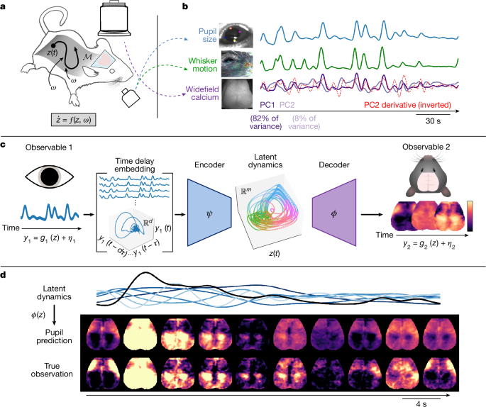
a, We performed simultaneous widefield optical imaging and face videography in awake mice. We interpreted these measurements as observations of dynamics on an organism-intrinsic arousal manifold \({\mathcal{M}}\) (that is, a low-dimensional surface within the state-space). Trajectories of the system state z along \({\mathcal{M}}\) reflect intrinsic arousal dynamics and stochastic (that is, arousal independent) perturbations ω(t) arising from within and outside the organism, such that \(\mathop{z}\limits^{.}=f(z,\omega )\). The silhouette of the mouse was adapted from ref. ⁷¹ and obtained from SciDraw (https://SciDraw.io) under a Creative Commons licence CC BY 4.0. b, We extracted three observables: scalar indices of pupil diameter and whisker motion, and high-dimensional images of widefield calcium fluorescence. Here widefield images are represented via the first two principal components (PCs). The first brain PC (PC1; dark purple) closely tracked pupil diameter and whisker motion and accounted for 70–90% of the variance in each mouse (Supplementary Fig. 1). However, remaining PCs often retained clear temporal relationships with the first; here, for instance, the temporal derivative of PC2 (red dashed line) closely resembles PC1 (Pearson r = −0.73), implying that nonlinear relationships with arousal dynamics extend beyond the dominant ‘arousal component’^2,44. c, We developed an approach to model the full manifestations of arousal dynamics. Each observable y_i is interpreted as resulting from an observation function of the latent arousal dynamics plus observable-specific variability η_i (that is, y_i = g_i(z) + η_i). By Takens’ theorem⁶, the full-state latent dynamics can, in principle, be recovered from a time delay embedding of a scalar observable. Accordingly, we learned an encoder ψ that maps from an embedding comprising d time-lagged copies of y₁ (that is, pupil diameter) to an m-dimensional latent space (m < d), as well as a decoder (ϕ) implementing a time-invariant mapping from this latent space to widefield measurements. Figure adapted from ref. ⁷², Oxford University Press. d, An example epoch contrasting original and pupil-reconstructed widefield images (test data from one mouse). The black trace indicates pupil diameter. The blue traces denote delay coordinates, where increasing lightness indicates increasing order (Methods).

Such a dominant explanatory factor for global covariance has been widely interpreted to reflect ‘arousal’, conventionally understood as a unidimensional continuum indexing the overall ‘wakefulness’ or ‘activation’ level of an organism^23,26. Crucially, this framing tacitly assumes that brain activity naturally decomposes into linearly independent factors. This, in turn, compels ad hoc explanations for the remaining, orthogonal dimensions of neural data—that is, by construction, ‘not arousal’ (for example, see refs. ^2,3,4).

A key caveat of this framing is that linear dimensions need not correspond to physically meaningful variables. More fundamentally, linear independence—although mathematically convenient—is biologically arbitrary and does not imply physical or mechanistic separability^45,46 (also see ref. ⁴⁷, chapter 6). Consistent with this, we observed that higher principal components typically retained clear temporal relationships to the first principal component, often closely approximating its successive time derivatives (Fig. 1b). These dynamical relationships support our alternative view: that scalar indices of ‘arousal’, such as pupil size or a single principal component, are best understood as one-dimensional projections of an underlying process (Fig. 1a), one whose full manifestations span and fundamentally entangle multiple (Euclidean) dimensions. Below, we elaborate on this perspective before introducing a dynamical systems framework enabling its empirical validation.

We interpret nominally arousal-related observables (for example, pupil size and whisking) as reflections of an organism-wide regulatory process (Fig. 1a). This dynamic regulation⁴⁸ may be viewed as a low-dimensional process whose evolution induces stereotyped variations in the high-dimensional state of the organism. Physiologically, this abstraction captures the familiar ability of arousal shifts to elicit multifaceted, coordinated changes throughout the organism (for example, ‘fight-or-flight’ versus ‘rest-and-digest’ modes)⁴⁹. Operationally, this framing motivates a separation between the effective dynamics of this system, which evolve along a latent, low-dimensional manifold^50,51, and the high-dimensional ‘observation’ space, which we express via time-invariant mappings from the latent manifold. In this way, rather than assuming high-dimensional, pairwise interactions among the measured variables, we attempted to parsimoniously attribute widespread variance to a common, latent dynamical system⁵².

To specify the instantaneous latent arousal state, we draw on Takens’ embedding theorem⁶ and connections with modern Koopman operator theory⁴², which together provide general conditions under which the embedding of a scalar time series in time delay coordinates can faithfully represent latent dynamics on the original, full-state attractor. As we hypothesized that brain-wide physiology is spatiotemporally regulated in accordance with these arousal dynamics⁹, this theory yields a surprising empirical prediction: a scalar observable of arousal dynamics (for example, pupil diameter) can suffice to reconstruct the states of a high-dimensional observable of brain physiology (for example, optical images of cortex-wide activity), insofar as both reflect the same underlying dynamics^7,53.

To test this hypothesis, we developed a data-driven framework to relate observables evolving under a shared dynamical system (Fig. 1c). For each mouse, we embedded pupil diameter in a high-dimensional space defined by its past values (that is, time delay coordinates). We learned a map (or encoder) ψ from this space to a continuous, low-dimensional latent space in which the instantaneous arousal state z is represented as a single point. We also learned a map (decoder) ϕ from this latent space to the widefield calcium observation space. These mappings, estimated with linear or nonlinear methods, together enable each calcium image to be expressed as a function of a multidimensional state inferred from pupil delay coordinates, to the extent that both observables are deterministically linked to the same latent state.

For all analyses, we focused on (‘infra-slow’⁵⁴) fluctuations below 0.2 Hz to distinguish arousal-related dynamics from physiologically distinct processes manifesting at higher frequencies (for example, delta waves)^55,56. To model the hypothesized mappings, we implemented an iterative, leave-one-out strategy in which models were trained using 10-min recordings concatenated across six mice, then tested on the held-out 10-min recording from the seventh mouse (Methods). Results from a separate, within-mouse train–test pipeline are shown in Supplementary Fig. 2.

For both pipelines, candidate models included a linear regression model based on a single lag-optimized copy of pupil diameter (‘no embedding’), as well as a model incorporating multiple delay coordinates and nonlinear mappings (‘latent model’). Both models allowed us to assess the hypothesis that the widefield measurements primarily reflect arousal-related variation. However, the latter model enables stronger validation of our framework by allowing detection of the hypothesized nonlinear, dynamical aspects of pupil-widefield covariation. Nonlinear mappings were learned through feedforward neural networks modelled after a variational autoencoder (Methods). See Extended Data Figs. 1 and 2 and Supplementary Text for validation on a toy (stochastic Lorenz) system.

Modelling results from the leave-one-out pipeline are shown in Fig. 2. We first considered total variance explained, summarized across time points and pixels. In each of n = 7 mice, our models reconstructed 60–85% of the total widefield variance below 0.2 Hz based on simultaneously recorded pupil diameter (Fig. 2a). This total variance was dominated by the first principal component (Supplementary Fig. 1), which showed a tight, linear relationship with pupil diameter, allowing much of it to be captured by a one-dimensional pupil regressor (Fig. 2a). These results thus support the notion that widefield calcium measurements are dominated by nominally arousal-related fluctuations. Nonetheless, as the total variance metric collapses across pixels and time points, we next examined whether model reconstructions faithfully captured geometric and dynamical structure within the original widefield data.

Fig. 2: Pupil diameter enables reconstruction of spatiotemporal brain dynamics.

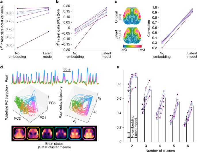
a,b, Variance explained in held-out widefield data from each of n = 7 mice (for each prediction, the model was trained on data from the other 6 mice). A simple linear regression model based on one (lag-optimized) pupil regressor (no embedding) accurately predicted approximately 70–85% of total variance in six of the seven mice (a). Delay embedding and non-linearities (latent model) further improved widefield prediction (a), crucially, doing so by reliably capturing variance orthogonal to PC1 (that is, PCs 2-N) that was not tracked by the scalar pupil regressor (b). See Extended Data Fig. 5 for pixelwise maps of variance explained. c, Reconstructing propagation dynamics. Phase maps were obtained from dynamic mode decomposition applied to the original and reconstructed data from n = 7 mice, and subsequently compared via (circular) spatial correlation. Phase maps from one example mouse are shown on the left (phase maps from the one-dimensional model are not shown, as they lack phase structure due to the absence of complex-valued modes). The Allen Mouse Common Coordinate Framework atlas is overlaid in white. d, Example state trajectories (held-out data) visualized in coordinates defined by pupil diameter (top), the first three widefield PCs (middle left) or three latent variables obtained from the delay-embedded pupil time series (middle right). Trajectories are colour coded by the cluster assignment of each time point as determined by a GMM applied to the original widefield image frames (middle left) or the same GMM applied to reconstructed frames (middle right) (k = 6 clusters; bottom). Cluster means are shown underneath. Similar colour arrangement within pupil delay coordinates indicates that pupil dynamics encode spatially specific information about cortex-wide activity. e, Decoding brain states from pupil dynamics. Comparison of decoder accuracy in properly identifying ground-truth GMM cluster assignments for each frame based on the most frequent assignment (‘null’ decoder) or on data reconstructed via either the no embedding or latent model.

Crucially—and in contrast to the no embedding model—the latent model captured substantial variance orthogonal to the first PC (Fig. 2b, Extended Data Figs. 3 and 4 and Supplementary Fig. 2). Spatially, the topography of total variance explained closely mirrored the first PC and was heavily weighted towards posteromedial cortices (Extended Data Fig. 5), resembling previous arousal-related maps^1,3,12,57. By contrast, the latent model additionally explained variance in anterolateral (‘orofacial’) cortices (Extended Data Fig. 5). These regions were more strongly correlated with pupil derivative and amplitude envelope (Extended Data Fig. 6), two features implicitly represented in the delay embedding and known to track neuromodulator dynamics^20,58. These modelling improvements did not trivially result from increased model complexity, as confirmed by shuffling pupil and widefield measurements across mice (Extended Data Fig. 7). We conclude that multiple widefield dimensions maintain lawful, time-invariant relationships with pupil dynamics.

These relationships imply that pupil and widefield measurements share latent, nonlinear geometric structure, consistent with both reflecting the structured flow of an underlying process. This interpretation would further predict that pupil dynamics encode the spatiotemporal dynamics of widefield calcium signals. To test this hypothesis, we fitted linear dynamical systems models (via dynamic mode decomposition⁴²; Methods) to the original and reconstructed datasets and examined the leading spatial modes. In all seven mice, the original widefield data yielded a complex-valued leading mode that indicated a cortex-wide propagation pattern resembling previous results^55,59. Crucially, the latent model consistently preserved this phase structure (Fig. 2c). By contrast, the no embedding model lacked spatiotemporal dynamics altogether (Supplementary Videos 1 and 2). Indeed, bona fide spatiotemporal dynamics are inherently multidimensional, as they entail interregional phase shifts that reside in the complex plane, thus requiring at least two (Euclidean) dimensions; by contrast, a one-dimensional system cannot generate or represent rich phase structure. Hidden Markov model analyses similarly supported the unique ability of delay embeddings to preserve widefield dynamical structure (Extended Data Fig. 8). Collectively, these points suggest that infra-slow widefield spatiotemporal dynamics reflect a multidimensional process that is also tracked by pupil dynamics.

Next, we sought to verify the continuous nature of this coupling by evaluating frame-by-frame spatial correspondence between the original and reconstructed datasets. To do this, we clustered variance-normalized image frames based on spatial similarity using a Gaussian mixture model (GMM), then quantified the percentage of ‘ground truth’ GMM cluster assignments (from the original data) matching those decoded by applying the same GMM to the reconstructed frames. Figure 2e shows the resulting accuracy as a function of the number of clusters.

Spatial patterns largely alternated between two main topographies, consistent with infra-slow spatiotemporal dynamics across modalities and species^9,30,57. With a two-cluster solution, the latent model enabled accurate decoding of more than 80% of image frames. Although accuracy gradually declined with increasing cluster number—reflecting reduced distinctiveness among clusters—it consistently improved from the null to the no embedding decoder, and, finally, to the latent model decoder. The latter uniquely tracked spatial variation along multiple dimensions; accordingly, its improvements became even more pronounced when clustering based on equally weighted principal components (Extended Data Fig. 9). Decoding improvements were also more apparent when labelling states according to an hidden Markov model (which also considers dynamics) rather than a GMM (Extended Data Fig. 8). These results confirm that pupil dynamics reliably and continuously index the instantaneous spatial topography of widefield calcium.

Beyond neuronal activity per se, spatially structured fluctuations are also prominent in metabolic and haemodynamic measurements. Such fluctuations are typically attributed to state-dependent, region-dependent and context-dependent responses to local neuronal signalling. By contrast, our account posits that multiple aspects of physiology are jointly regulated according to arousal dynamics (see also, for example, refs. ^27,44). This suggests the possibility of more parsimoniously relating multiple spatiotemporal readouts of brain physiology.

To test this prediction, we leveraged two readouts acquired alongside neuronal calcium using the multispectral optical imaging platform⁵: oxidative metabolism (indexed by flavoprotein autofluorescence (FAF)⁵) and haemodynamic signals (which approximate the physiological basis of fMRI). We attempted to reconstruct all three observables from delay embedded pupil measurements. To do this, we froze the encoder ψ trained to predict calcium, and simply trained two new decoders to map from its latent space to FAF and oxygenated haemoglobin (ϕ₂ and ϕ₃ in Fig. 3a, respectively).

Fig. 3: Multimodal measurements reconstructed from a shared latent manifold.

a, Delay embedding framework extended to multimodal observables. We coupled the existing encoder—trained to predict calcium images—to decoders trained separately to predict FAF and haemoglobin. ox., oxidative. b, Example reconstructions of widefield calcium (jRGECO fluorescence), metabolism (FAF) and blood oxygen (concentration of oxygenated haemoglobin). c, Reconstruction performance (as in Fig. 2a,b). See Extended Data Fig. 10 for pixelwise maps of variance explained (n = 7 mice).

Modelling results are shown in Fig. 3b. As with calcium, we successfully modelled the majority of variance in these two modalities across all n = 7 mice. Both modalities were dominated by the first principal component, but slightly less so than calcium (Supplementary Figs. 3 and 4; compare with Supplementary Fig. 1). Correspondingly, delay embeddings and nonlinearities made even larger contributions to the total explained variance in these two modalities, even after adjusting for a modality-specific, globally optimized delay (Fig. 3c and Extended Data Fig. 10). We conclude that a far larger portion of metabolic and haemodynamic fluctuations is attributable to a common, arousal-related mechanism than conventionally appreciated (also see refs. ^9,37). For context, predictions based on pixelwise calcium signals are shown in Supplementary Fig. 5. We return to the physiological implications of these relationships in the Discussion.

A key motivation for our framework is the growing array of observables linked to arousal indices^15,27, despite persistent ambiguity surrounding this construct²⁹. Accordingly, we next considered how our framing of arousal could quantitatively integrate such findings. We extended our approach to publicly available behavioural and electrophysiological recordings from the Allen Institute Brain Observatory⁸. We examined 30-min recordings from mice in a task-free context, deriving eight common indices of brain state (Methods): pupil diameter, running speed, the hippocampal θ:δ ratio, instantaneous rate of hippocampal sharp-wave ripples (SWRs), band-limited power (BLP) derived from the local field potential across visual cortical regions, and mean firing rate across several hundred neurons per mouse. BLP was analysed within three canonical frequency ranges: 0.5–4 Hz (‘delta’), 3–6 Hz (‘alpha’⁶⁰) and 40–100 Hz (‘gamma’).

We began by concatenating measurements across mice, then trained neural networks to predict each observable from a latent space constructed from delay embedded pupil measurements. Next, we applied the learned encoding to the delay embedded pupil measurements for each individual, training decoders to map from this shared latent space to the observables of the individual (see Supplementary Fig. 6 for quantitative validation). Finally, we repeated this procedure for the primary widefield dataset, thus leveraging pupil diameter as a common reference to align observables across individuals and datasets to a shared manifold.

To visualize the resulting, multidataset generative model (Fig. 4), we defined the arousal manifold \({\mathcal{M}}\) as a two-dimensional latent space and evaluated each observable’s mapping ϕ_i over a grid of sample points within it. We also computed a vector field f(z) over this grid using a data-driven analytic representation of the latent dynamics⁶¹ (Methods). Thus, at each point along \({\mathcal{M}}\), Fig. 4 depicts the conditional expectation of both the local direction of arousal dynamics (via f) and the state of each observable y_i (via ϕ_i). \({\mathcal{M}}\), f and the mappings \({\{{\phi }_{i}\}}_{i=1}^{N}\) together constitute our dynamical, relational interpretation of arousal.

Fig. 4: Unifying observables through arousal dynamics.

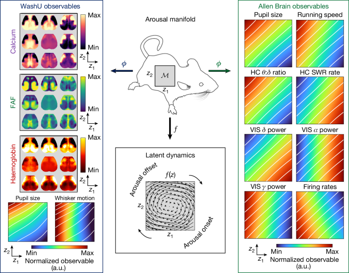
The arousal manifold provides an organism-intrinsic reference frame to align and aggregate measurements across datasets. To visualize the discovered relations, we define the manifold as a two-dimensional latent space parameterized by abstract coordinates z₁ and z₂ (that is, \({\bf{z}}\in {\mathcal{M}}\subset {{\mathbb{R}}}^{2}\); top middle). The learned decoders ϕ map each point z in this manifold (that is, each latent arousal state) to an expected value of a particular observable (for example, a single widefield calcium image or a single value of pupil size), enabling representations of the manifold from the perspective of various observables (left and right columns). Here widefield observables are evaluated at 3 × 3 evenly spaced points within the latent space, whereas each scalar observable is evaluated over a 100 × 100 grid. The white diagonals indicate iso-contours of pupil size in either the WashU or Allen Brain Observatory datasets, providing a shared visual reference across observables within the same dataset. Meanwhile, f(z), which we approximate via a data-driven analytic representation⁶¹, maps each point z to an expected direction of movement (that is, \(\mathop{{\bf{z}}}\limits^{.}=f({\bf{z}})\)), enabling representation of the vector field over the manifold (bottom middle). Together, these representations convey how a typical trajectory on the arousal manifold, governed by intrinsic dynamics, maps onto observable changes. a.u., arbitrary units; HC, hippocampus; VIS, visual cortex. The silhouette of the mouse was adapted from ref. ⁷¹ and obtained from SciDraw (https://scidraw.io) under a Creative Commons licence CC BY 4.0.

This representation unifies and clarifies themes across the experimental literature, which we briefly summarize here. As expected, running speed, the hippocampal θ:δ ratio, cortical gamma BLP and mean firing rate are all positively correlated with pupil size along a single, principal dimension, z₁ (that is, the horizontal coordinate in each plot; Fig. 4, ‘Allen Brain observables’). These observables are inversely correlated with delta BLP, alpha BLP and hippocampal SWR rate along the same dimension, each of which indexes more internally oriented processes that are enhanced during sensory disengagement^16,26.

Including a second dimension (z₂, vertical coordinate in each plot) reveals a rotational flow that recapitulates observations relating to brain and behavioural state transitions^20,58,62,63. Thus, the ‘arousal onset’ (Fig. 4) begins with decreasing alpha BLP⁶³, followed by increases in firing rates and gamma BLP and, subsequently, pupil diameter^44,62. This phase is accompanied by the onset of whisking and cortical propagation towards midline and posterior regions^55,57 (widefield optical imaging (WashU) observables). Continuing clockwise, pupil diameter, locomotion and the hippocampal θ:δ ratio peak around the time that alpha BLP begins to increase from its nadir, consistent with its appearance at the offset of locomotion⁶⁰ (Fig. 4, ‘arousal offset’). Increases in delta BLP and hippocampal SWR rate ensue, in parallel with cortical propagation from posteromedial to anterolateral regions (WashU observables). This embedding of cortex-wide topographical maps within a canonical ‘arousal cycle’ resembles previous findings in humans and monkeys, which also describe topographically parallel waves in subcortical structures⁹.

In summary, this framework parsimoniously and quantitatively represents a globally coordinated pattern that is registered only piecemeal through diverse observables. Although verification would ideally require simultaneous measurements of all observables—which remains practically infeasible—the ability to integrate partial observations has a key role in contextualizing results and supporting experiment–theory iteration.

The concept of ‘brain state’ has gained prominence in systems neuroscience as experimental advances have made studies in awake, behaving organisms increasingly routine¹⁵. Although brain state is typically viewed as comprising several biological or behavioural factors—one of which is often presumed to be ‘arousal’^4,12—principled criteria for defining and disentangling such components are lacking. Alternatively, construing organisms as dynamical systems^52,64, our approach seeks to factorize brain (or rather, organismal) state in terms of constituent endogenous processes, one of which, examined herein, we identified with the arousal construct. Despite grounding arousal in a specific process, our results reveal this process to be multidimensionally structured and nonlinearly coupled to various observables, ultimately implying even broader relevance for arousal than presently recognized.

This generalized view of arousal resonates with two emerging themes. First, brain or arousal states often correspond to qualitatively distinct (neuro-)physiological regimes^27,65, limiting the utility of simply orthogonalizing observations with respect to an arousal index (for example, via linear regression or removal of the leading principal component). Second, numerous studies have reported non-random transitions among brain states¹², as well as functional correlates of dynamical indices of arousal, such as the phase or derivative of pupil size^44,58,62, often with surprising timescale invariance^9,17,56. These observations imply an underlying nonlinear dynamic system⁶⁶. Together, these two themes portray arousal as a dynamic, pervasive and persistent ‘background’; this complicates the ability to interpret spontaneous or task-related^3,12 variation observed even over seconds without reference to this evolving internal context^13,65.

Indeed, by more rigorously capturing the scope of arousal dynamics, our models reveal surprisingly rich spatiotemporal structure across the cortex, challenging conventional views of the underlying mechanisms. Thus, for decades, large-scale brain dynamics have been overwhelmingly interpreted as summations of diverse interactions among discrete regions^10,11,40, fuelling a proliferation of decomposition techniques. Although distinctions among modalities and species should not be overlooked, evidence across these domains has increasingly converged towards a small set of core spatiotemporal components^30,36,38, alongside growing appreciation for arousal-related contributions^{28,31,32,35,40}. We extend these themes by advocating a more radically unified view: that these core components are themselves projections of a non-decomposable dynamical system—the same system that effectively underpins arousal. In this sense, arousal dynamics do not merely modulate interregional interactions, but actively generate spatiotemporal structure through the synchronized⁵³ propagation of topographically organized rotating waves⁹.

This unified model specifically concerns infra-slow dynamics. Although similar spatial patterns occur at timescales of greater than 1 Hz (ref. ⁶⁷)—probably reflecting shared anatomical constraints—dynamical behaviour more clearly distinguishes these two timescales^55,59, suggesting distinct generative mechanisms⁵⁶. Nonetheless, the expression of faster spatiotemporal dynamics is strongly modulated by infra-slow (and/or arousal) dynamics^54,55,67. Generalizing this theme, we suggest that the infra-slow evolution of arousal state modulates parameters governing faster processes throughout the brain and body (for example, Fig. 4).

This theoretical framing suggests a simplified view of the interrelations among electrical, metabolic and vascular cerebral activity. Tight coupling across these domains—essential for sustaining brain function—is typically attributed to complex neurometabolic and neurovascular cascades operating locally, thereby posing an enormous regulatory challenge. By contrast, longstanding evidence shows that neuromodulatory processes can influence these domains in parallel^68,69, suggesting mechanisms enabling their coordinated regulation. The strong performance of our model (Fig. 3) suggests that such mechanisms may be actively harnessed to effectively streamline cerebral regulation in accordance with arousal dynamics, thereby reducing reliance on conventional feedforward processes (for example, ‘the haemodynamic response’). This interpretation could help to explain observations that are difficult to reconcile with local response models (for example, ref. ⁷⁰), although its validation requires targeted experiments.

Finally, although we have adopted the term ‘arousal’ given its widespread use for the observables analysed here, we used it simply as a label for the latent process inferred from the observables in a data-driven manner. For the same reason, our results probably relate to a range of cognitive and behavioural phenomena traditionally distinguished from arousal (for example, ‘attention’), but potentially coupled to or overlapping with the dynamical process formalized here¹³.

Datasets and preprocessing

Dataset 1: WashU

Animal preparation. All procedures described below were approved by the Washington University Animal Studies Committee in compliance with the American Association for Accreditation of Laboratory Animal Care guidelines. Mice were raised in standard cages in a double-barrier mouse facility with a 12–12-h light–dark cycle and ad libitum access to food and water (22 °C ambient temperature and 40–60% humidity). Experiments used n = 7 12-week-old mice hemizygous for Thy1-jRGECO1a (JAX 030525) on a C57BL/6J background, enabling optical imaging of the jRGECO1a fluorescent calcium sensor protein primarily expressed in excitatory neurons of cortical layers 2/3 and 5 (ref. ⁷³). Before imaging, a cranial window was secured to the intact skull of each mouse with dental cement under isoflurane anaesthesia according to previously published protocols⁷².

Data acquisition. Widefield imaging was conducted on a dual fluorophore optical imaging system; details of this system have been presented elsewhere^5,74. In brief, sequential illumination was provided at 470 nm, 530 nm and 625 nm; reflected light in each channel was collected by a lens (focal length = 75 mm; NMV-75M1, Navitar), split by a 580-nm dichroic (FF580-FDi02-t3-25 × 36, Semrock) into two channels, one filtered by 500-nm long pass (FF01-500/LP-25, Semrock; blocks FAF excitation, passes FAF emission and 530-nm Hb reflectance), and the other by a 593-nm long pass (FF01-593/LP-25, Semrock; blocks jRGECO1a excitation, passes jRGECO1a emission and 625-nm Hb reflectance). The two channels were detected separately via two CMOS cameras (Zyla 5.5, Andor). Data were cropped to 1,024 × 1,024 pixels, and binned to 512 × 512 to achieve a frame rate of 100 Hz in each camera, with all contrasts imaged at 25 Hz. The light-emitting diodes (LEDs) and camera exposures were synchronized and triggered via a data acquisition card (PCI-6733, National Instruments) using MATLAB R2019a (MathWorks).

Mice were head fixed under the imaging system objective using an aluminium bracket attached to a skull-mounted Plexiglas window. Before data acquisition in the awake state, mice were acclimated to head fixation over several days.

The body of the mouse was supported by a felt pouch suspended by optical posts (Thorlabs). Resting-state imaging was performed for 10 min in each mouse. Before each imaging run, dark counts were imaged for each mouse for 1 s with all LEDs off to remove background sensor noise.

Preprocessing. Images were spatially normalized, downsampled to 128 × 128 pixels, co-registered and affine transformed to the Paxinos atlas, temporally detrended (fifth order polynomial fit) and spatially smoothed (5 × 5 pixel Gaussian filter with standard deviation of 1.3 pixels)⁷⁵. Changes in 530-nm and 625-nm reflectance were interpreted using the modified Beer–Lambert law to calculate changes in oxy-haemoglobin and deoxy-haemoglobin concentration⁵.

Image sequences of fluorescence emission detected by CMOS1 (that is, uncorrected FAF) and CMOS2 (that is, uncorrected jRGECO1a) were converted to percent change (dF/F) by dividing the time trace of each pixel by its average fluorescence over each imaging run. Absorption of excitation and emission light for each fluorophore due to haemoglobin was corrected as outlined in ref. ⁷⁶. From the face videography, we derived scalar indices of pupil size via DeepLabCut software⁷⁷ and whisker motion via the Lucas–Kanade optical flow method⁷⁸ applied to and subsequently averaged across five manually selected data points on the whiskers. The resulting pupil diameter, whisker motion and widefield time series were bandpass filtered between 0.01 < f < 0.2 Hz to distinguish the hypothesized spatiotemporal process from distinct phenomena occurring at higher frequencies (for example, slow waves)⁵⁵, and to accommodate finite scan duration for 10 min. For visualization only—namely, to view the Allen atlas boundaries in register with cortical maps—we manually aligned the Paxinos-registered data from one mouse to a 2D projection of the Allen Mouse Common Coordinate Framework (v3)⁷⁹ using four anatomical landmarks: the left, right and midline points at which the anterior cortex meets the olfactory bulbs, and an additional midline point at the base of the retrosplenial cortex^3,80. Coordinates obtained from this transformation were used to overlay the Common Coordinate Framework boundaries onto the Paxinos-registered cortical maps for all mice.

Dataset 2: Allen Brain Observatory

We additionally analysed recordings obtained from awake mice and publicly released via the Allen Brain Observatory Neuropixels Visual Coding project⁸. These recordings include eye-tracking, running speed (estimated from running wheel velocity), and high-dimensional electrophysiological recordings obtained with Neuropixels probes⁸¹. We restricted analyses to the ‘functional connectivity’ stimulus set, which included a 30-min ‘spontaneous’ session with no overt experimental stimulation. Data were accessed via the Allen Software Development Kit (https://allensdk.readthedocs.io/en/latest/). From 26 available recording sessions, we excluded four with missing or compromised eye-tracking data, one lacking local field potential (LFP) data, and five with locomotion data indicating a lack of immobile periods or appearing otherwise anomalous, thus leaving a total of n = 16 recordings for downstream analyses.

Preprocessing. From the electrophysiological data, we derived estimates of population firing rates and several quantities based on the LFP. We accessed spiking activity as already extracted by Kilosort2 (ref. ²). Spikes were binned in 1.2-s bins as previously described², and a mean firing rate was computed across all available units from neocortical regions surpassing the default quality control criteria. Neocortical LFPs were used to compute BLP within three canonical frequency bands: gamma (40−100 Hz), ‘alpha’ (3−6 Hz) and delta (0.5−4 Hz). Specifically, we downsampled and low passed the signals with a 100-Hz cutoff, computed the spectrogram (scipy.signal.spectrogram⁸²) at each channel in sliding windows of 0.5 s with 80% overlap, and averaged spectrograms across all channels falling within ‘VIS’ regions (including primary and secondary visual cortical areas). BLP was then computed by integrating the spectrogram within the frequency bands of interest and normalizing by the total power. A similar procedure was applied to LFP recordings from the hippocampal CA1 region to derive estimates of hippocampal theta (5−8 Hz) and delta (0.5−4 Hz) BLP. Hippocampal SWRs were detected on the basis of the hippocampal CA1 LFP via an automated algorithm⁸³ following previously described procedures⁸⁴. In general, extreme outlying values (generally artefact) were largely mitigated through median filters applied to all observables, whereas an additional thresholding procedure was used to interpolate over large negative transients in running speed. Finally, all time series were downsampled to a sampling rate of 20 Hz and filtered between 0.01 < f < 0.2 Hz to facilitate integration with dataset 1.

Data analysis

State-space framework

Formally, we considered the generic state-space model:

where the nonlinear function f determines the (nonautonomous) flow of the latent (that is, unobserved), vector-valued arousal state \({\bf{z}}={[{z}_{1},{z}_{2},\ldots ,{z}_{m}]}^{{\rm{T}}}\) along a low-dimensional attractor manifold \({\mathcal{M}}\), whereas ω(t) reflects random (external or internal) perturbations decoupled from f that nonetheless influence the evolution of z (that is, ‘dynamical noise’). We consider our N observables \({\{{{\bf{y}}}_{i}\}}_{i=1}^{N}\) as measurements of the arousal dynamics, each resulting from an observation equation g_i, along with other contributions η_i(t) that are decoupled from the dynamics of z (and in general are unique to each observable). Thus, in this framing, samples of the observable y_i at consecutive time points t and t + 1 are linked through the evolution of the latent variable z as determined by f. Note that f is presumed to embody various causal influences spanning both brain and body (and the feedback between them), whereas measurements (of either brain or body) y_i do not contribute to these dynamics. This framework provides a formal, data-driven approach to parsimoniously capture the diverse manifestations of arousal dynamics, represented by the proportion of variance in each observable y_i that can be modelled purely as a time-invariant mapping from the state-space of z.

State-space reconstruction via delays

Our principal task was to learn a mapping from arousal-related observables to the multidimensional space where the hypothesized arousal process evolves in time. To do this, we took advantage of Takens’ embedding theorem from dynamical systems theory, which has been widely used for the purpose of nonlinear state-space reconstruction from an observable. Given p snapshots of the scalar observable y in time, we began by constructing the following Hankel matrix \({\bf{H}}\in {{\mathbb{R}}}^{d\times (p-d+1)}\):

for p time points and d time delays. Each column of H represents a short trajectory of the scalar observable y(t) over d time points, which we refer to as the delay vector h(t). These delay vectors represent the evolution of the observable within an augmented, d − dimensional state-space.

We initially constructed H as a high-dimensional (and rank-deficient) matrix to ensure it covered a sufficiently large span to embed the manifold. We subsequently reduced the dimensionality of this matrix to improve conditioning and reduce noise. Dimensionality reduction is carried out in two steps: (1), through projection onto an orthogonal set of basis vectors (below), and (2) through nonlinear dimensionality reduction via a neural network (detailed in the next section).

For the initial projection, we note that the leading left eigenvectors of H converge to Legendre polynomials in the limit of short delay windows⁸⁵. Accordingly, we used the first r = 10 discrete Legendre polynomials as the basis vectors of an orthogonal projection matrix:

(polynomials obtained from the special.legendre function in SciPy⁸²). We applied this projection to the Hankel matrix constructed from a pupil diameter timecourse. The resulting matrix \(\mathop{{\bf{Y}}}\limits^{ \sim }\in {{\mathbb{R}}}^{r\times (p-d+1)}\) is given by:

Each column of this matrix, denoted \(\widetilde{{\bf{y}}}={{\bf{P}}}^{(r){\rm{T}}}{\bf{h}}\), represents the projection of a delay vector h(t) onto the leading r Legendre polynomials. The components of this state vector, \(\widetilde{{\bf{y}}}(t)={[{y}_{0}(t),\ldots ,{y}_{r-1}(t)]}^{{\rm{T}}}\), are the individual r Legendre coordinates⁸⁵, which form the input to the neural network encoder.

The dimensionality of H is commonly reduced through its singular value decomposition (SVD; for example, see refs. ^43,86). In practice, we found that projection onto Legendre polynomials yields marginal improvements over SVD of H, particularly in the low-data limit⁸⁵. More importantly, the Legendre polynomials additionally provided a universal, analytic basis in which to represent the dynamics; this property was exploited for comparisons across mice and datasets.

Choice of delay embedding parameters was guided on the basis of autocorrelation time and attractor reconstruction quality (that is, unfolding the attractor while maximally preserving geometry), following decomposition of H. The number of delay coordinates was guided based on asymptoting reconstruction performance using a linear regression model. For all main text analyses, the Hankel matrix was constructed with d = 100 time delays, with each row separated by Δt = 3 time steps (equivalently, adopting H as defined in equation (3), we set d = 300 and subsampled every third row). As all time series were analysed at a sampling frequency of 20 Hz, this amounts to a maximum delay window of 100 × 3 × 0.05 = 15 s.

For all modelling, pupil diameter was first shifted in time to accommodate any physiological delay between the widefield signals and the pupil. For each widefield modality, this time shift was selected as the abscissa corresponding to the peak of the cross-correlation function between the pupil and the mean widefield signal. For the leave-one-out pipeline, we used the median time shift across the six mice in the training set.

State-space mappings via VAE

To interrelate observables through this state-space framework (and thus, through arousal dynamics), we ultimately sought to approximate the target functions

where h_i(t) represents the delay vectors (columns of the Hankel matrix constructed from a scalar observable y_i), \({\bf{z}}(t)\in {{\mathbb{R}}}^{m}\) is the low-dimensional representation of the latent arousal state, and y_j(t) is a second observable. Various linear and nonlinear methods can be used to approximate these functions (for example, see ref. ⁸⁷). Our primary results were obtained through a probabilistic modelling architecture based on the variational autoencoder (VAE)^88,89.

In brief, a VAE is a deep generative model comprising a pair of neural networks (that is, an encoder and decoder) that are jointly trained to map data observations to the mean and variance of a latent distribution (via the encoder), and to map random samples from this latent distribution back to the observation space (decoder). Thus, the VAE assumes that data observations y are taken from a distribution over some latent variable z, such that each data point is treated as a sample \(\widehat{z}\) from the prior distribution p_θ(z), typically initialized according to the standard diagonal Gaussian prior, that is, \({p}_{\theta }(z)={\mathcal{N}}(z| 0,{\bf{I}})\). A variational distribution q_φ(z∣y) with trainable weights φ is introduced as an approximation to the true (but intractable) posterior distribution p(z∣y).

As an autoencoder, q_φ(z∣y) and p_θ(y∣z) encode observations into a stochastic latent space, and decode from this latent space back to the original observation space. The training goal is to maximize the marginal likelihood of the observables given the latent states z. This problem is made tractable by instead maximizing an evidence lower bound, such that the loss is defined in terms of the negative evidence lower bound:

where the first term corresponds to the log-likelihood of the data (reconstruction error), and the Kullback–Leibler (KL) divergence term regularizes the distribution of the latent states q_φ(z∣y) to be close to that of the prior p_θ(z). Under Gaussian assumptions, the first term is simply obtained as the mean squared error, that is, \(\parallel y-\widehat{y}{\parallel }_{2}^{2}\). The KL term is weighted according to an additional hyperparameter β, which controls the balance between these two losses^90,91. Model parameters (φ and θ) can be jointly optimized via stochastic gradient descent through the reparameterization trick⁸⁸.

In the present framework, rather than mapping back to the original observation space, we used the decoder p_θ(y∣z) to map from z to a new observation space. In this way, we used a probabilistic encoder and decoder, respectively, to approximate our target functions ψ(h) (which is partly constituted by the intermediate projection P^(r), via equation (5)) and ϕ(z). Of note, VAE training incorporates stochastic perturbations to the latent representation, thus promoting discovery of a smooth and continuous manifold. Such a representation is desirable in the present framework, such that changes within the latent space (which is based on the delay coordinates) are smoothly mapped to changes within the observation spaces⁹². After training, to generate predicted trajectories, we simply fed the mean output from the encoder (that is, q(μ_z∣y)) through the decoder to (deterministically) generate the maximum a posteriori estimate.

Model architecture and hyperparameters

VAE models were trained with the Adam optimizer⁹³ (see Supplementary Table 1 for details specific to each dataset). Across datasets, the encoder comprised a single-layer feedforward neural network with \(\tanh \) activations, which transformed the vector of leading Legendre coordinates \(\widetilde{{\bf{y}}}\) (equation (5)) to (the mean and log variance of) an m-dimensional latent space (m = 4 unless otherwise stated). The latent space Gaussian was initialized with a noise scale of σ = 0.1 to stabilize training. The decoder from this latent space included a single-layer feedforward neural network consisting of 10 hidden units with \(\tanh \) activations, followed by a linear readout layer matching the dimensionality of the target signal. During training, the KL divergence weight was gradually annealed to a factor of β over the first approximately 15% of training epochs to mitigate posterior collapse^90,94. Hyperparameters pertaining to delay embedding and the VAE were primarily selected by examining expressivity and robustness within the training set of a subset of mice. Within each modelling pipeline or dataset, hyperparameters were kept fixed across all mice and modalities to mitigate overfitting.

Model training pipeline

For all main analyses, we implemented an iterative leave-one-out strategy in which candidate models were trained using 10-min recordings concatenated across six of the seven mice, and subsequently tested on the held-out 10-min recording obtained from the seventh mouse. To make model training efficient, we used a randomized SVD approach^95,96. Thus, for each iteration, we began by pre-standardizing (to zero mean and unit variance) all datasets (‘standardization 1’) and aligning in time following delay embedding of the pupil measurements (thus removing the initial time points of the widefield data for which no delay vector of pupil values was available). Next, we lag adjusted the (delay embedded) pupil and widefield time series from each mouse according to the median lag (across the six training mice) derived from the cross-correlation function of each training mouse between their pupil time series and their mean widefield signal. Next, we concatenated the six training datasets and computed the SVD of the concatenated widefield time series (\({{\bf{Y}}}_{{\rm{cat}}}={{\bf{U}}}_{{\rm{cat}}}{{\bf{S}}}_{{\rm{cat}}}{{\bf{V}}}_{\,{\rm{cat}}}^{{\rm{T}}}\)) to obtain group-level spatial components V_cat. Data were projected onto the leading ten components (that is, the first ten columns of V_cat) and standardized once more (‘standardization 2’), and training proceeded within this reduced subspace. Note that this group-level subspace excluded data from the test mouse, such that V_cat differed for each iteration of the leave-one-out pipeline.

For the held-out mouse, the pre-standardized pupil diameter (that is, having undergone ‘standardization 1’ above) was standardized once more using the training set parameters (‘standardization 2’), and used to generate a prediction within the group-level 10-dimensional subspace. This prediction was then inverse transformed and unprojected back into the high-dimensional image space using the standardization and projection parameters of the training set. All model evaluations were performed following one final inverse transformation to undo the initial pre-standardization (standardization 1), enabling evaluation in the original dF/F units. The pre-standardization parameters were not predicted from the training data; including the pre-standardization as part of the model would make model performance sensitive to the robustness of the relationship between dF/F values and raw pupil units, which is not scientifically relevant in this context. Finally, any subsequent projections used to evaluate model performance in terms of principal components (as in Fig. 2b) utilized mouse-specific SVD modes (denoted simply as V), rather than the group modes (V_cat) used during training.

In addition to the leave-one-out pipeline, we implemented a separate, within-subject pipeline in which we trained models on the first 5 min of data for each mouse and report model performance on the final 3.5 min of the 10-min session. This training pipeline involved prediction of the full-dimensional images, without the intermediate SVD used in the leave-one-out pipeline. All results pertaining to this modelling pipeline are contained in Supplementary Fig. 2.

Model evaluation

For analyses reporting ‘total variance’ explained (Figs. 2a and 3c, top), we report the R² value over the full 128 × 128 image, computed across all held-out time points. R² was computed as the coefficient of determination, evaluated over all pixels n and temporal samples t (that is, the total variance):

where y_n,t and \({\widehat{y}}_{n,t}\) are, respectively, the true and predicted values of y at the n-th pixel and t-th time point, and \(\bar{y}\) is the global mean. In practice, this value was computed as the pixel-wise weighted average of R² scores, with weights determined by pixel variance (computed using the built-in function sklearn.metrics.r2_score, with ‘multioutput’ set to ‘variance weighted’).

To examine variance explained beyond the first principal component (Figs. 2b and 3c, bottom), we computed the (randomized) SVD of the widefield data for each mouse (Y = USV^T) and, after training, projected the original and reconstructed widefield data onto the top N = 200 spatial components excluding the first (that is, YV_2:N) before computing R² values. The matrices from this SVD were used for all analyses involving projection onto the leading principal components.

For the shuffled control analysis (Extended Data Fig. 7), we examined total variance explained in widefield data from the test set (as in Fig. 2a), except that for each mouse, we swapped the original pupil diameter timecourse with one from each of the other six mice (that is, we shuffled pupil diameter and widefield calcium data series across mice).

Dynamic mode decomposition

Dynamic mode decomposition (DMD)^97,98,99 is a data-driven method to dimensionally reduce time series measurements into a superposition of spatiotemporal modes. Given the time series matrix Y = {y(t₁), y(t₂), …, y(t_p)}, where y(t_i) represents the system state vector at the i-th time point, the data are split into two matrices, Y⁽¹⁾ = {y(t₁), …, y(t_p−1)} and Y⁽²⁾ = {y(t₂), …, y(t_p)}. DMD seeks an approximate linear mapping A such that

Theoretically, the operator A represents a low-rank approximation to an infinite-dimensional linear operator—namely, the Koopman operator—associated with nonlinear systems^42,99, motivating the use of DMD even in the context of nonlinear dynamics. This low-rank approximation is obtained via SVD of Y⁽¹⁾ and Y⁽²⁾. The measurement data can thus be approximated in terms of the spectral decomposition of A:

where the eigenvectors v_k give the dominant spatial modes, the eigenvalues ω_k give the dominant temporal frequencies and the coefficients b_k determine the amplitudes.

For each mouse, we applied DMD separately to three data matrices: the original widefield calcium images, and the predictions generated through both the no embedding model and the latent model. Here again, for numerical efficiency, we incorporated randomized SVD as part of the randomized DMD algorithm¹⁰⁰ implemented in pyDMD^101,102.

Following application of DMD, we constructed spatial phase maps from the leading eigenvector of each A matrix. Specifically, given the leading eigenvector \({{\bf{v}}}_{1}={[{v}_{1},{v}_{2},\ldots ,{v}_{n}]}^{{\rm{T}}}\in {{\mathbb{C}}}^{n}\), we computed the phase at each pixel i as \({\theta }_{i}=\arg ({v}_{i})\), where \(\arg (\,\cdot \,)\) denotes the complex argument of each entry, and v_i represents the value of the eigenvector v₁ at the i-th pixel. Note that the no embedding model predictions yielded exclusively real-valued eigenvectors, as these model predictions were fundamentally rank-one (that is, they reflect linear transformations of the scalar pupil diameter). Accordingly, as the complex argument maps negative real numbers to 0 and positive real numbers to π, phase maps obtained from the no embedding model predictions were restricted to these two values.

We used the circular correlation coefficient to quantify the similarity between the phase map obtained from the original dataset and the phase map obtained from either of the two model predictions. Specifically, let θ_i and \({\widehat{\theta }}_{i}\) represent the phase at spatial location i in the phase maps of the original and reconstructed datasets. The circular correlation ρ_circ between the two phase maps was computed as¹⁰³:

where \(\bar{\theta }\) and \(\bar{\widehat{\theta }}\) are the mean phase angles (that is, the mean directions) of the respective maps. The circular correlation is bounded between −1 and 1, where 1 indicates perfect spatial phase alignment between the datasets, and −1 indicates an inverted pattern. However, because the eigenvectors are only determined up to a complex sign, Fig. 2c reports the absolute value this quantity, that is, ∣ρ_circ∣.

Clustering and decoding analysis

We used GMMs to assign each (variance-normalized) image frame to one of k clusters (parameterized by the mean and covariance of a corresponding multivariate Gaussian) in an unsupervised manner. This procedure enables assessment of the spatial specificity of cortical patterns predicted by arousal dynamics, with increasing number of clusters reflecting increased spatial specificity.

In brief, a GMM models the observed distribution of feature values x as coming from some combination of k Gaussian distributions:

where μ_i and Σ_i are the mean and covariance matrix of the i-th Gaussian, respectively, and π_i is the probability of x belonging to the i-th Gaussian (that is, the Gaussian weight). We fit the mean, covariance and weight parameters through the standard expectation-maximization algorithm as implemented in the GMM package available in scikit-learn¹⁰⁴. This procedure results in a posterior probability for each data point’s membership to each of the k Gaussians (also referred to as the ‘responsibility’ of Gaussian i for the data point); (hard) clustering can then be performed by simply assigning each data point to the Gaussian cluster with maximal responsibility.

Images were spatially normalized such that the (brain-masked) image at each time point was set to unit variance (thus yielding a ‘spatial sign’¹⁰⁵), followed by projection onto the top three principal components to regularize the feature space. Then, for each mouse and each number of clusters k, a GMM with full covariance prior was fit to the normalized, dimensionally reduced image frames to obtain a set of ‘ground-truth’ cluster assignments. After training, this GMM was subsequently applied to the reconstructed rather than the original image frames to obtain maximum a posteriori cluster assignments associated with the no embedding or latent model predictions. These cluster assignments were compared with the ground-truth assignments, with accuracy computed as the proportion of correctly identified cluster labels.

The preceding algorithm effectively clusters the dimensionally reduced image frames on the basis of their cosine distance (technically, their L₂-normalized Euclidean distance). Because the first principal component tends to explain the vast majority of the variance, this Euclidean-based distance is largely determined by distance along the leading dimension. This analysis choice suffices for the primary purpose of the analysis—namely, to assess correspondence between the original and reconstructed data at the level of individual time points. However, in the context of multivariate data, it is common to also normalize the data features before clustering, thus equally weighting each (spatial) dimension of the data. To examine this clustering alternative, we performed feature-wise normalization of each spatial dimension following projection of the (sample-wise) normalized image frames onto the top three principal components. This essentially constitutes a whitening transformation of the image frames, with Euclidean distance in this transformed space effectively approximating the Mahalanobis distance between image frames. Clustering results from this procedure are shown in Extended Data Fig. 9. For these supplementary analyses, which we also extend to higher cluster numbers, we used a spherical (rather than full) covariance prior as additional regularization.

Hidden Markov model

We additionally used hidden Markov models (HMMs) to capture the temporal dynamics within the original and reconstructed widefield calcium measurements. In brief, under a Gaussian HMM, the observations {y(t₁), y(t₂), …, y(t_p)} are assumed to be generated by a sequence of latent discrete states z_t ∈ {1, …, K}, with the full generative model including:

1. (1)

   A transition matrix \({\bf{A}}\in {{\mathbb{R}}}^{K\times K}\), where A_ij = P(z_t + 1 = j∣z_t = i) represents the probability of transitioning from state i to state j.

2. (2)

   An initial state distribution, represented as a vector of state probabilities \({\boldsymbol{\pi }}\in {{\mathbb{R}}}^{K}\) (with π_i = P(z₁ = i)).

3. (3)

   Emission distributions, such that each observation y_t is modelled as a multivariate Gaussian conditioned on the latent state z_t—that is, \({{\bf{y}}}_{t} \sim {\mathcal{N}}({{\boldsymbol{\mu }}}_{z},{{\boldsymbol{\Sigma }}}_{z})\), where μ_z and Σ_z denote the state-specific mean and covariance, respectively.

The model is thus parameterized by \({\boldsymbol{\theta }}=\{{\bf{A}},{\boldsymbol{\pi }},{\{{{\boldsymbol{\mu }}}_{z},{{\boldsymbol{\Sigma }}}_{z}\}}_{z=1}^{K}\}\). We estimated these parameters via an expectation-maximization algorithm (Baum-Welch), as implemented in hmmlearn¹⁰⁶.

Before HMM fitting, the widefield images were projected onto the three leading principal components and normalized along each dimension (similar to preprocessing for the GMM with whitening above, but without the initial normalization of each individual image frame). HMMs were fit to these data for a range of state numbers (K = 2, 3, 4, 5, 6).

To ensure a robust fit, we initialized the state probabilities to be uniform, \({{\rm{\pi }}}_{i}=\frac{1}{K}\), and initialized the transition matrix with probabilities of 0.8 along the diagonal (that is, within-state transitions or ‘stay’ probabilities) and 0.2/K for all off-diagonal elements (that is, between-state transitions).

An HMM was first fit to the original data (yielding a ground-truth model), and then separate HMMs were fit to the reconstructions. In the latter cases, the emission parameters \({\{{{\boldsymbol{\mu }}}_{z},{{\boldsymbol{\Sigma }}}_{z}\}}_{z=1}^{K}\) were fixed to the values obtained from the ground-truth model, so that only the transition matrix A and the initial state probabilities π were updated.

For each mouse and each choice of K states, we computed three evaluation metrics:

1. (1)

   The log-likelihood of the observed data under the fitted HMMs.

2. (2)

   Decoding accuracy, computed as the agreement between the latent states inferred from the ground-truth HMM and those predicted by the HMMs fit to the reconstructed datasets.

3. (3)

   Transition matrix similarity, which we computed as the row-wise KL divergence between the ground-truth and the reconstructed transition matrices:

   $${\mathbb{KL}}({{\bf{A}}}_{{\rm{true}}}\parallel {{\bf{A}}}_{{\rm{model}}})=\frac{1}{K}\mathop{\sum }\limits_{i=1}^{K}\mathop{\sum }\limits_{j=1}^{K}{A}_{ij}^{{\rm{true}}}\log \frac{{A}_{ij}^{{\rm{true}}}}{{A}_{ij}^{{\rm{model}}}}.$$

   (14)

   For numerical stability in computing KL divergence, transition probabilities below a threshold of ϵ = 10⁻⁶ were set to zero and each row was renormalized to maintain stochasticity, that is,

   $$\mathop{\sum }\limits_{j=1}^{K}{A}_{ij}=1\quad \,{\rm{for\; all}}\,i.$$

   (15)

Multi-dataset integration

To extend our framework to an independent set of observables, we trained our architecture on concatenated time series from the Allen Institute Brain Observatory dataset (n = 16 mice). For visualization purposes, we sought to learn a group-level two-dimensional embedding (that is, \({\bf{z}}\in {{\mathbb{R}}}^{2}\)) based on delay embedded pupil measurements. After group-level training, we froze the weights of the encoder and retrained the decoders independently for each mouse, enabling individual-specific predictions for the Allen Institute mice from a common (that is, group-level) latent space. We additionally applied these encoder weights to delay embedded pupil observations from the original ‘WashU’ dataset, once again retraining mouse-specific decoders to reconstruct observables from the common latent space.

Once trained, this procedure results in the generative model p(y_i, z), which we used to express the posterior probability of each observable y_i as a function of position within a common 2D latent space (note that this formulation does not seek a complete generative model capturing all joint probabilities among the observables). This allowed us to systematically evaluate the conditional expectation (\({\mathbb{E}}({{\bf{y}}}_{i}| {\bf{z}})\)) for each observable over a grid of points in the latent space, which was regularized to be continuous (roughly, an isotropic Gaussian⁸⁹). Figure 4 represents this expectation, averaged over decoder models trained for each mouse.

To visualize a vector field over the manifold, we applied a data-driven nonlinear equation discovery method—sparse identification of nonlinear dynamics (SINDy)^61,107—to the dynamics represented in the 2D latent coordinates, treating data from each mouse as an independent trajectory. We obtained a simple nonlinear oscillator:

with α = 0.384, β = −0.251 and γ = −0.193. This system was evaluated over a grid of evenly spaced sample points within the latent space, enabling a visual approximation of the true underlying vector field.

Reporting summary

Further information on research design is available in the Nature Portfolio Reporting Summary linked to this article.

All analysis code for this study is publicly available on GitHub (https://github.com/ryraut/arousal_dynamics).

References

Author notes

1. Ryan V. Raut

   Present address: Mallinckrodt Institute of Radiology, Washington University in St. Louis, St. Louis, MO, USA

Authors and Affiliations

1. Allen Institute, Seattle, WA, USA

   Ryan V. Raut

2. Department of Physiology & Biophysics, University of Washington, Seattle, WA, USA

   Ryan V. Raut

3. Department of Psychiatry, Perelman School of Medicine, University of Pennsylvania, Philadelphia, PA, USA

   Zachary P. Rosenthal

4. Mallinckrodt Institute of Radiology, Washington University in St. Louis, St. Louis, MO, USA

   Xiaodan Wang, Marcus E. Raichle & Adam Q. Bauer

5. Department of Neurology, Washington University in St. Louis, St. Louis, MO, USA

   Hanyang Miao, Jin-Moo Lee & Marcus E. Raichle

6. Department of Computer Science & Engineering, University of California San Diego, La Jolla, CA, USA

   Zhanqi Zhang

7. Department of Mechanical Engineering, University of Washington, Seattle, WA, USA

   Steven L. Brunton

8. Department of Biology, University of Washington, Seattle, WA, USA

   Bingni W. Brunton

9. Department of Applied Mathematics, University of Washington, Seattle, WA, USA

   J. Nathan Kutz

Contributions

R.V.R., Z.P.R., S.L.B., B.W.B. and J.N.K. conceptualized the study. Z.P.R. acquired the data. Z.P.R., H.M. and Z.Z. processed the data. R.V.R. analysed the data and undertook the modelling. R.V.R., Z.P.R., X.W., J.-M.L., M.E.R., A.Q.B., S.L.B. and J.N.K. provided resources and funding. R.V.R. wrote and revised the manuscript with input from all authors.

Corresponding author

Correspondence to Ryan V. Raut.

Competing interests

The authors declare no competing interests.

Peer review information

Nature thanks Shella Keilholz and the other, anonymous, reviewer(s) for their contribution to the peer review of this work. Peer reviewer reports are available.

Open Access This article is licensed under a Creative Commons Attribution-NonCommercial-NoDerivatives 4.0 International License, which permits any non-commercial use, sharing, distribution and reproduction in any medium or format, as long as you give appropriate credit to the original author(s) and the source, provide a link to the Creative Commons licence, and indicate if you modified the licensed material. You do not have permission under this licence to share adapted material derived from this article or parts of it. The images or other third party material in this article are included in the article’s Creative Commons licence, unless indicated otherwise in a credit line to the material. If material is not included in the article’s Creative Commons licence and your intended use is not permitted by statutory regulation or exceeds the permitted use, you will need to obtain permission directly from the copyright holder. To view a copy of this licence, visit http://creativecommons.org/licenses/by-nc-nd/4.0/.

Reprints and permissions

References

Shimaoka, D., Harris, K. D. & Carandini, M. Effects of arousal on mouse sensory cortex depend on modality. Cell Rep. 22, 3160–3167 (2018).
Stringer, C. et al. Spontaneous behaviors drive multidimensional, brainwide activity. Science 364, eaav7893 (2019).
Musall, S., Kaufman, M. T., Juavinett, A. L., Gluf, S. & Churchland, A. K. Single-trial neural dynamics are dominated by richly varied movements. Nat. Neurosci. 22, 1677–1686 (2019).
Kaplan, H. S. & Zimmer, M. Brain-wide representations of ongoing behavior: a universal principle? Curr. Opin. Neurobiol. 64, 60–69 (2020).
Wang, X. et al. Spatiotemporal relationships between neuronal, metabolic, and hemodynamic signals in the awake and anesthetized mouse brain. Cell Rep. 43, 114723 (2024).
Takens, F. Detecting strange attractors in turbulence. Lecture Notes Math. 898, 366–381 (1981).
Sugihara, G. et al. Detecting causality in complex ecosystems. Science 338, 496–500 (2012).
Siegle, J. H. et al. Survey of spiking in the mouse visual system reveals functional hierarchy. Nature https://doi.org/10.1038/s41586-020-03171-x (2021).
Raut, R. V. et al. Global waves synchronize the brain’s functional systems with fluctuating arousal. Sci. Adv. 7, eabf2709 (2021).
Cabral, J., Kringelbach, M. L. & Deco, G. Functional connectivity dynamically evolves on multiple time-scales over a static structural connectome: models and mechanisms. NeuroImage 160, 84–96 (2017).
Suárez, L. E., Markello, R. D., Betzel, R. F. & Misic, B. Linking structure and function in macroscale brain networks. Trends Cogn. Sci. 24, 302–315 (2020).
McCormick, D. A., Nestvogel, D. B. & He, B. J. Neuromodulation of brain state and behavior. Annu. Rev. Neurosci. 43, 391–415 (2020).
Buzsáki, G. The Brain from Inside Out (Oxford Univ. Press, 2019).
Raichle, M. E. The restless brain: how intrinsic activity organizes brain function. Phil. Trans. R. Soc. B 370, 20140172 (2015).
Greene, A. S., Horien, C., Barson, D., Scheinost, D. & Constable, R. T. Why is everyone talking about brain state? Trends Neurosci. https://doi.org/10.1016/j.tins.2023.04.001 (2023).
Liu, X., Leopold, D. A. & Yang, Y. Single-neuron firing cascades underlie global spontaneous brain events. Proc. Natl Acad. Sci. USA 118, e2105395118 (2021).
Crombie, D., Spacek, M. A., Leibold, C. & Busse, L. Spiking activity in the visual thalamus is coupled to pupil dynamics across temporal scales. PLoS Biol. 22, e3002614 (2024).
Drew, P. J., Winder, A. T. & Zhang, Q. Twitches, blinks, and fidgets: important generators of ongoing neural activity. Neuroscientist 25, 298–313 (2019).
Zagha, E. et al. The importance of accounting for movement when relating neuronal activity to sensory and cognitive processes. J. Neurosci. 42, 1375–1382 (2022).
Collins, L., Francis, J., Emanuel, B. & McCormick, D. A. Cholinergic and noradrenergic axonal activity contains a behavioral-state signal that is coordinated across the dorsal cortex. eLife 12, e81826 (2023).
Lohani, S. et al. Spatiotemporally heterogeneous coordination of cholinergic and neocortical activity. Nat. Neurosci. 25, 1706–1713 (2022).
Bechtel, W. & Abrahamsen, A. in Philosophy of Complex Systems: Volume 10 of Handbook of the Philosophy of Science (ed. Hooker, C.) 257–285 (Elsevier, 2011).
Duffy, E. The psychological significance of the concept of “arousal” or “activation”. Psychol. Rev. 64, 265–275 (1957).
Kahneman, D. Attention and Effort (Prentice-Hall, 1973).
Andrew, R. J. Arousal and the causation of behaviour. Behaviour 51, 135–165 (1974).
McGinley, M. et al. Waking state: rapid variations modulate neural and behavioral responses. Neuron 87, 1143–1161 (2015).
Rasmussen, R., O’Donnell, J., Ding, F. & Nedergaard, M. Interstitial ions: a key regulator of state-dependent neural activity? Prog. Neurobiol. 193, 101802 (2020).
Martin, C. G., He, B. J. & Chang, C. State-related neural influences on fMRI connectivity estimation. NeuroImage 244, 118590 (2021).
Grujic, N., Polania, R. & Burdakov, D. Neurobehavioral meaning of pupil size. Neuron https://doi.org/10.1016/j.neuron.2024.05.029 (2024).
Gutierrez-Barragan, D., Ramirez, J. S. B., Panzeri, S., Xu, T. & Gozzi, A. Evolutionarily conserved fMRI network dynamics in the mouse, macaque, and human brain. Nat. Commun. 15, 8518 (2024).
Shine, J. M. Neuromodulatory influences on integration and segregation in the brain. Trends Cogn. Sci. 23, 572–583 (2019).
Shahsavarani, S. et al. Cortex-wide neural dynamics predict behavioral states and provide a neural basis for resting-state dynamic functional connectivity. Cell https://doi.org/10.1016/j.celrep.2023.112527 (2023).
Benisty, H. et al. Rapid fluctuations in functional connectivity of cortical networks encode spontaneous behavior. Nat. Neurosci. 27, 148–158 (2024).
Turchi, J. et al. The basal forebrain regulates global resting-state fMRI fluctuations. Neuron 97, 940–952.e4 (2018).
Bolt, T. et al. Autonomic physiological coupling of the global fMRI signal. Nat. Neurosci. https://doi.org/10.1038/s41593-025-01945-y (2025).
Matsui, T., Murakami, T. & Ohki, K. Transient neuronal coactivations embedded in globally propagating waves underlie resting-state functional connectivity. Proc. Natl Acad. Sci. USA 113, 6556–6561 (2016).
Chen, J. E. et al. Resting-state ‘physiological networks’. NeuroImage 213, 116707 (2020).
Bolt, T. et al. A parsimonious description of global functional brain organization in three spatiotemporal patterns. Nat. Neurosci. 25, 1093–1103 (2022).
Pang, J. C. et al. Geometric constraints on human brain function. Nature 618, 566–574 (2023).
Pais-Roldán, P. et al. Contribution of animal models toward understanding resting state functional connectivity. NeuroImage 245, 118630 (2021).
Strogatz, S. H. Nonlinear Dynamics and Chaos: with Applications to Physics, Biology, Chemistry, and Engineering 2nd edn (CRC Press, 2019).
Brunton, S. L., Budišić, M., Kaiser, E. & Kutz, J. N. Modern Koopman theory for dynamical systems. SIAM Rev. 64, 229–340 (2022).
Brunton, S. L., Brunton, B. W., Proctor, J. L., Kaiser, E. & Kutz, J. N. Chaos as an intermittently forced linear system. Nat. Commun. 8, 19 (2017).
Reitman, M. E. et al. Norepinephrine links astrocytic activity to regulation of cortical state. Nat. Neurosci. 26, 579–593 (2023).
Dyer, E. L. & Kording, K. Why the simplest explanation isn’t always the best. Proc. Natl Acad. Sci. USA 120, e2319169120 (2023).
Meilă, M. & Zhang, H. Manifold learning: what, how, and why. Annu. Rev. Stat. Appl. 11, 393–417 (2024).
Gould, S. J. The Mismeasure of Man 1st edn (Norton, 1981).
Bich, L., Mossio, M., Ruiz-Mirazo, K. & Moreno, A. Biological regulation: controlling the system from within. Biol. Phil. 31, 237–265 (2016).
Berntson, G. G., Cacioppo, J. T. & Quigley, K. S. Autonomic determinism: the modes of autonomic control, the doctrine of autonomic space, and the laws of autonomic constraint. Psychol. Rev. 98, 459–487 (1991).
Schöner, G. & Kelso, J. A. S. Dynamic pattern generation in behavioral and neural systems. Science 239, 1513–1520 (1988).
Haken, H. Information and Self-Organization (Springer, 2006).
Bertalanffy, L. v. General System Theory: Foundations, Development, Applications 2nd edn (George Braziller, 1969).
Rulkov, N. F., Sushchik, M. M., Tsimring, L. S. & Abarbanel, H. D. I. Generalized synchronization of chaos in directionally coupled chaotic systems. Phys. Rev. E 51, 980–994 (1995).
Palva, J. M. & Palva, S. Infra-slow fluctuations in electrophysiological recordings, blood-oxygenation-level-dependent signals, and psychophysical time series. NeuroImage 62, 2201–2211 (2012).
Mitra, A. et al. Spontaneous infra-slow brain activity has unique spatiotemporal dynamics and laminar structure. Neuron 98, 297–305.e6 (2018).
Okun, M., Steinmetz, N. A., Lak, A., Dervinis, M. & Harris, K. D. Distinct structure of cortical population activity on fast and infraslow timescales. Cereb. Cortex 29, 2196–2219 (2019).
Barson, D. et al. Simultaneous mesoscopic and two-photon imaging of neuronal activity in cortical circuits. Nat. Methods 17, 107–113 (2020).
Reimer, J. et al. Pupil fluctuations track rapid changes in adrenergic and cholinergic activity in cortex. Nat. Commun. 7, 13289 (2016).
Vanni, M. P., Chan, A. W., Balbi, M., Silasi, G. & Murphy, T. H. Mesoscale mapping of mouse cortex reveals frequency-dependent cycling between distinct macroscale functional modules. J. Neurosci. 37, 7513–7533 (2017).
Nestvogel, D. B. & McCormick, D. A. Visual thalamocortical mechanisms of waking state-dependent activity and alpha oscillations. Neuron 110, 120–138.e4 (2022).
Brunton, S. L., Proctor, J. L. & Kutz, J. N. Discovering governing equations from data by sparse identification of nonlinear dynamical systems. Proc. Natl Acad. Sci. USA 113, 3932–3937 (2016).
Article ADS MathSciNet CAS PubMed PubMed Central Google Scholar
Reimer, J. et al. Pupil fluctuations track fast switching of cortical states during quiet wakefulness. Neuron 84, 355–362 (2014).
Liu, X. et al. Arousal transitions in sleep, wakefulness, and anesthesia are characterized by an orderly sequence of cortical events. NeuroImage 116, 222–231 (2015).
Varela, F. J., Thompson, E. & Rosch, E. The Embodied Mind: Cognitive Science and Human Experience (MIT Press, 1991).
Sadeh, S. & Clopath, C. Contribution of behavioural variability to representational drift. eLife 11, e77907 (2022).
Schreiber, T. & Schmitz, A. Surrogate time series. Phys. D Nonlinear Phenom. 142, 346–382 (2000).
Chan, A. W., Mohajerani, M. H., LeDue, J. M., Wang, Y. T. & Murphy, T. H. Mesoscale infraslow spontaneous membrane potential fluctuations recapitulate high-frequency activity cortical motifs. Nat. Commun. 6, 7738 (2015).
Raichle, M. E., Hartman, B. K., Eichling, J. O. & Sharpe, L. G. Central noradrenergic regulation of cerebral blood flow and vascular permeability. Proc. Natl Acad. Sci. USA 72, 3726–3730 (1975).
Lou, H. C., Edvinsson, L. & MacKenzie, E. T. The concept of coupling blood flow to brain function: revision required? Ann. Neurol. 22, 289–297 (1987).
Zhang, Q. et al. Cerebral oxygenation during locomotion is modulated by respiration. Nat. Commun. 10, 5515 (2019).
Mouse silhouette. Zenodo https://doi.org/10.5281/zenodo.3925991 (2020).
Rosenthal, Z. P. et al. Local perturbations of cortical excitability propagate differentially through large-scale functional networks. Cereb. Cortex 30, 3352–3369 (2020).
Dana, H. et al. Thy1 transgenic mice expressing the red fluorescent calcium indicator jRGECO1a for neuronal population imaging in vivo. PLoS ONE 13, e0205444 (2018).
Padawer-Curry, J. A. et al. Psychedelic 5-HT2a receptor agonism: neuronal signatures and altered neurovascular coupling. Preprint at bioRxiv https://doi.org/10.1101/2023.09.23.559145 (2023).
White, B. R. et al. Imaging of functional connectivity in the mouse brain. PLoS ONE 6, e16322 (2011).
Ma, Y. et al. Wide-field optical mapping of neural activity and brain haemodynamics: considerations and novel approaches. Phil. Trans. R. Soc. B 371, 20150360 (2016).
Mathis, A. et al. DeepLabCut: markerless pose estimation of user-defined body parts with deep learning. Nat. Neurosci. 21, 1281–1289 (2018).
Lucas, B. D. & Kanade, T. An iterative image registration technique with an application to stereo vision. In Proc. 7th International Joint Conference on Artificial Intelligence Vol. 2, 674–679 (Morgan Kaufmann Publishers, 1981).
Wang, Q. et al. The Allen Mouse Brain Common Coordinate Framework: a 3D reference atlas. Cell 181, 936–953.e20 (2020).
Saxena, S. et al. Localized semi-nonnegative matrix factorization (LocaNMF) of widefield calcium imaging data. PLoS Comput. Biol. 16, e1007791 (2020).
Jun, J. J. et al. Fully integrated silicon probes for high-density recording of neural activity. Nature 551, 232–236 (2017).
Virtanen, P. et al. SciPy 1.0: fundamental algorithms for scientific computing in Python. Nat. Methods 17, 261–272 (2020).
Denovellis, E. Eden-Kramer-lab/ripple_detection: v1.2.0. Zenodo https://zenodo.org/records/7011175 (2022).
Kay, K. et al. A hippocampal network for spatial coding during immobility and sleep. Nature 531, 185–190 (2016).
Gibson, J. F., Doyne Farmer, J., Casdagli, M. & Eubank, S. An analytic approach to practical state space reconstruction. Phys. D Nonlinear Phenom. 57, 1–30 (1992).
Broomhead, D. & King, G. P. Extracting qualitative dynamics from experimental data. Phys. D Nonlinear Phenom. 20, 217–236 (1986).
Abarbanel, H. D. I., Carroll, T. A., Pecora, L. M., Sidorowich, J. J. & Tsimring, L. S. Predicting physical variables in time-delay embedding. Phys. Rev. E 49, 1840–1853 (1994).
Kingma, D. P. & Welling, M. Auto-encoding variational Bayes. Preprint at https://arxiv.org/abs/1312.6114 (2014).
Kingma, D. P. & Welling, M. An Introduction to Variational Autoencoders (Now Foundations and Trends, 2019).
Sønderby, C. K., Raiko, T., Maaløe, L., Sønderby, S. K. & Winther, O. Ladder variational autoencoders. in Advances in Neural Information Processing Systems 29 (NIPS 2016) (eds Lee, D. et al.) (Curran Associates, 2016).
Higgins, I. et al. beta-VAE: learning basic visual concepts with a constrained variational framework. In International Conference on Learning Representations (ICLR, 2022).
Casdagli, M., Eubank, S., Farmer, J. D. & Gibson, J. State space reconstruction in the presence of noise. Phys. D Nonlinear Phenom. 51, 52–98 (1991).
Kingma, D. P. & Ba, J. Adam: a method for stochastic optimization. Preprint at https://arxiv.org/abs/1412.6980 (2017).
Bowman, S. R. et al. Generating sentences from a continuous space. in Proc. 20th SIGNLL Conference on Computational Natural Language Learning (eds Riezler, S. & Goldberg, Y.) 10–21 (Association for Computational Linguistics, 2016).
Halko, N., Martinsson, P. G. & Tropp, J. A. Finding structure with randomness: probabilistic algorithms for constructing approximate matrix decompositions. SIAM Rev. 53, 217–288 (2011).
Brunton, S. L. & Kutz, J. N. Data-Driven Science and Engineering: Machine Learning, Dynamical Systems, and Control 2nd edn (Cambridge Univ. Press, 2022).
Schmid, P. J. Dynamic mode decomposition of numerical and experimental data. J. Fluid Mech. 656, 5–28 (2010).
Kutz, J. N., Brunton, S. L., Brunton, B. W. & Proctor, J. L. Dynamic Mode Decomposition: Data-Driven Modeling of Complex Systems (SIAM, 2016).
Colbrook, M. J. in Handbook of Numerical Analysis Vol. 25 (eds Mishra, S. & Townsend, A.) 127–230 (Elsevier, 2024).
Erichson, N. B., Mathelin, L., Kutz, J. N. & Brunton, S. L. Randomized dynamic mode decomposition. SIAM J. Appl. Dyn. Syst. 18, 1867–1891 (2019).
Demo, N., Tezzele, M. & Rozza, G. PyDMD: Python dynamic mode decomposition. J. Open Source Softw. 3, 530 (2018).
Ichinaga, S. M. et al. PyDMD: a Python package for robust dynamic mode decomposition. J. Mach. Learn. Res. 25, 1–9 (2024).
Jammalamadaka, S. R. & Sarma, Y. R. in Statistical Theory and Data Analysis II (ed. Matusita, K.) 349–364 (Elsevier, 1988).
Pedregosa, F. et al. Scikit-learn: machine learning in Python. J. Mach. Learn. Res. 12, 2825–2830 (2011).
Serneels, S., De Nolf, E. & Van Espen, P. J. Spatial sign preprocessing: a simple way to impart moderate robustness to multivariate estimators. J. Chem. Inf. Model. 46, 1402–1409 (2006).
hmmlearn. GitHub https://github.com/hmmlearn/hmmlearn (2025).
Kaptanoglu, A. et al. PySINDy: a comprehensive Python package for robust sparse system identification. J. Open Source Softw. 7, 3994 (2022).
Raut, R., Rosenthal, Z., Wang, X. & Bauer, A. Simultaneous widefield optical imaging of cortex-wide calcium, metabolism, and hemodynamics, with pupil and whisker motion. Zenodo https://doi.org/10.5281/zenodo.15777664 (2025).
Schneider, M. et al. Spontaneous pupil dilations during the resting state are associated with activation of the salience network. NeuroImage 139, 189–201 (2016).
Lazari, A. et al. The mouse motor system contains multiple premotor areas and partially follows human organizational principles. Cell Rep. https://doi.org/10.1016/j.celrep.2024.114191 (2024)
Acknowledgements
We thank the Allen Institute for the publicly available data used in this study; and T. Voss for assistance with the optical set-up. The mouse illustration in Figs. 1 and 4 is adapted from ref. 71, obtained from SciDraw (https://SciDraw.io). R.V.R. was supported by the Shanahan Family Foundation Fellowship at the Interface of Data and Neuroscience at the Allen Institute and the University of Washington, supported in part by the Allen Institute. This research was additionally supported by the American Heart Association grant 20PRE34990003 (to Z.P.R.); the US National Institutes of Health grants R01NS126326, R01NS102870 and RF1AG07950301 (to A.Q.B.), and R37NS110699, R01NS084028 and R01NS094692 (to J.-M.L.); and the National Science Foundation AI Institute in Dynamic Systems grant 2112085 (to J.N.K. and S.L.B.).
Ethics declarations