Citizen science illuminates the nature of city lights

Artificial light is now widely recognized as an important environmental pollutant^1,2, affecting about a quarter of Earth’s land surface and 88% of Europe³. Despite this, the character of the sources of light emissions, particularly in cities, remains poorly understood as public inventories lack information about sources other than streetlights (for example, signs and decorative lights). This information cannot be directly determined from aerial or satellite views (Fig. 1) because of insufficient sensitivity and spatial resolution. We addressed this knowledge gap by co-designing a citizen science⁴ app called Nachtlichter⁵ (night-time lights) and using it to observe and classify the different types of light sources visible from public spaces. Our main goals were to examine the relative frequencies of lights present at different levels of urbanization and how the absolute numbers of lights relate to radiance measured by satellites. This information is needed for effective targeting for lighting, energy and environmental policy and for modeling the environmental impacts of light pollution.

Fig. 1: Overhead views of an artificially lit area at night near Cologne, Germany, at different spatial scales.

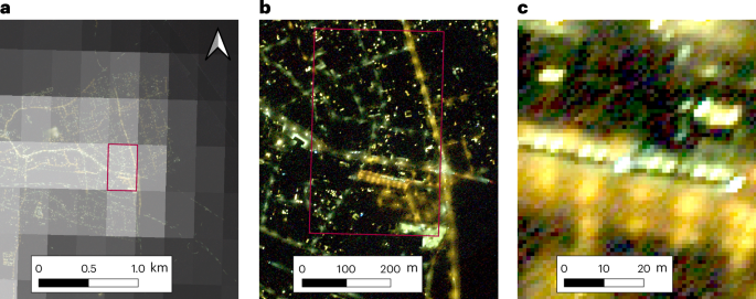
a, Low-resolution (750 m) satellite data from the Visible Infrared Imaging Radiometer Suite Day–Night Band (October 2018), with high-resolution aerial data in the background (taken 20 December 2021). b, The red rectangle highlights a single reprojected pixel (290 × 460 m), which is shown in greater detail on the aerial photographs (~1-m resolution). c, Further zoom, near the bottom right of the rectangle. While the positions of individual light sources can be identified, the type of light source (for example sign, floodlight) cannot be determined, even at this relatively high resolution.

Overhead images of cities at night (Fig. 1) emphasize street networks due to the viewing angle and suggest that public street lighting is the main or only relevant source of light from cities. Public authorities are responsible for streetlights, and with the rise of geographic information systems, have records of their locations and properties. Perhaps for these reasons, much of current lighting discussion and policy focuses on street lighting. Observational studies, however, have found the majority of light emissions from cities generally come from other sources⁵ (median 67%, range 25–92%). For example, an evaluation of light sources in Flagstaff, Arizona, USA, based on surveys, sampling and luminaire information, suggested that streetlights are responsible for only about 12% of upward escaping light emissions⁶. An intervention experiment in Tucson, Arizona, USA, found that streetlights were responsible for only 16% of the radiance in satellite observations taken after midnight⁷. The largest reported streetlight fraction was 75% for Ribeira, Spain, but even in this case, the same publication reported 45% after reconstruction of the lighting⁸. Comprehensive lighting inventories that identify all of the light sources have so far only been conducted in peacetime for areas with small numbers of lights, for example, in International Dark Sky Place applications^9,10 (a US Corps of Engineers study from 1943 provides a wartime example¹¹). An important question for anyone wishing to control urban light pollution is therefore ‘what makes up the rest of the light?’

Beyond policy, the lack of direct knowledge of light sources is problematic for several research areas. The contribution of light towards artificial skyglow above and near cities, for example, depends strongly on the direction of radiance³. Information about the typical distributions of light source type, color and degree of shielding are therefore critical inputs for skyglow models, which may strongly underestimate skyglow if they neglect sources other than streetlights¹². Relatedly, studies of lighting change based on late-night satellite observations suggest widespread but relatively slow global increase of about 2% annually^13,14, whereas early evening visual observations of stars by citizen scientists suggest a much more rapid annual increase of about 10% (ref. ¹⁵). This difference could potentially be explained by changes in the type, color and direction of lights active at different times of night¹⁶. However, without large-scale lighting inventories, it would be difficult to confirm or refute such a hypothesis.

Despite lacking understanding of the sources of light, the environmental, social and health consequences of lighting are increasingly clear¹⁷. For example, urban lights attract birds from large distances, often with deadly consequences^18,19. The artificial brightening of the night sky has altered Earth’s night environment over vast areas, extending far from cities³. Despite its comparatively weak illuminance, this skyglow has been shown to affect the behavior of wild animals²⁰. Laboratory studies suggest that even plants react to skies brighter than those under which life evolved²¹. Night-time light emissions are also directly linked to monetary and energy issues, as recently illustrated by temporary restrictions on outdoor light use enacted in Germany²² and other countries, following the Russian invasion of Ukraine. Light reductions therefore promote climate stability and biodiversity.

The Nachtlichter project aimed to obtain a basic empirical understanding of the character of lighting in cities and smaller settlements in Germany through citizen science supported by a mobile app. This methodology was ideal for allowing residents in multiple places to collect data during the same time period. In Nachtlichter, participants walked along a transect, usually from one street corner to the next, and counted and classified the light sources they observed according to 18 pre-defined categories (Methods and Fig. 2). Consistency between different observers was ensured through a mandatory online training²³. The standard deviation of variability in light counts between different observers on the same street was estimated to be roughly 10–20% (ref. ⁵), which is similar to the standard deviation of monthly radiance reported by the satellite sensor used in this study²⁴.

Fig. 2: The 18 different categories into which lights were classified.

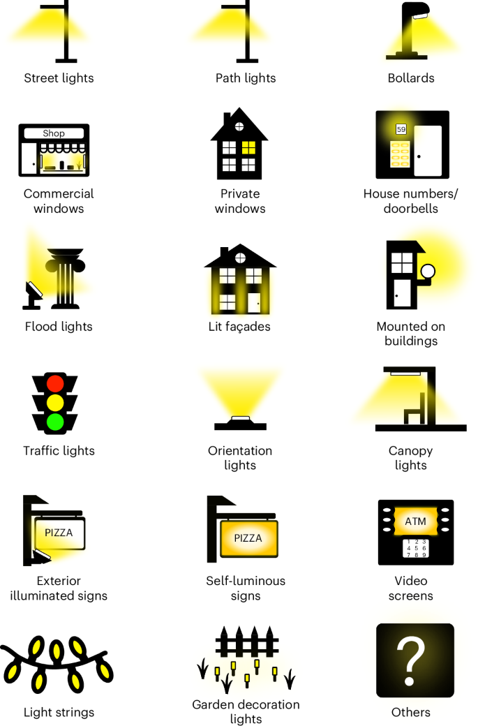
These and similar icons were used in the tutorial during training and in the app during data acquisition.

Observations were performed during autumn of 2021, and the study areas were designed to completely cover all publicly accessible areas within specified reprojected satellite pixels of the Visible Infrared Imaging Radiometer Suite Day–Night Band (DNB), a night-time lights observing satellite²⁵. As a German-speaking citizen science team, we had initially planned to cover a total of 6 km² in three German communities. However, the response was greater than expected, and we acquired data over a total area of roughly 22 km² in 33 communities, nine of which were outside of Germany⁵.

During 2021, a total of 234,044 lights were reported on 3,868 individual transects, by 258 registered participants during 4,409 observation surveys. The number of surveys exceeded the number of transects because some transects were surveyed multiple times. Private windows were the most frequently observed light type, followed by streetlights and commercial windows (Table 1). Five light categories were found to change considerably, depending on the time at which the transect was observed: private and commercial windows, signs (meaning the sum of the three sign categories shown in Fig. 2), canopy lights and lights mounted on buildings (Extended Data Fig. 8). A correction based on a logistic function was applied to estimate the number of active lights that would have been observed during early (19:00) or late (00:00) evening (Methods).

The radiance observed by satellite was positively correlated with the total number of light sources per km² (Fig. 3a; Spearman r = 0.67). This positive correlation was also observed for 17 of the 18 different light types (Spearman r from 0.3 to 0.65; Extended Data Figs. 1 and 2); only garden decoration lights exhibited a negative correlation (Spearman r = −0.15, p < 0.04). We find a median radiance of 1 nW cm⁻²sr⁻¹ per 317 counted lights per km² across all locations. When the entire dataset was treated as a single analysis area, the relationship was 302 counted lights per km². On the basis of our temporal correction and for Germany only, if all observations were made at 19:00, we would expect to have a relation of 385 ± 16 lights per km² per nW cm⁻²sr⁻¹ (standard errors) or 219 ± 11 lights per km² for observations at 00:00 (Supplementary Table 1 and Supplementary Figs. 1 and 2). For several light types, the counted number of lights was not proportional to the satellite radiance. For example, the density of street and path lights rises more slowly than the median value in the dataset, whereas the density of signs rises more quickly (Fig. 3). This is because the mix of lighting types differs between more and less urban areas, as discussed below. The relationship between lights expected at midnight and DNB radiance was considerably smaller (120 ± 6) for the areas surveyed outside of Germany, compared to those inside.

Fig. 3: Relationship between light density and satellite radiance.

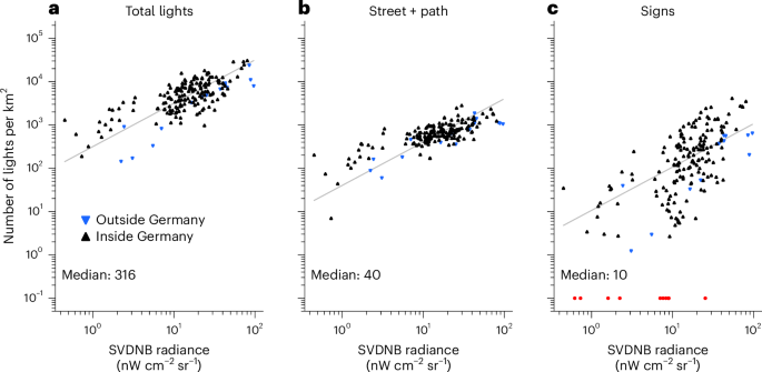
a–c, The relationship is shown for the sum of all lights (a), for the sum of street and path lights (b) and for the sum of the three sign categories (c). The line is not a fit but rather shows the median relationship over all analysis areas (both inside and outside of Germany). A time correction is not applied for these graphs; the results of multiple surveys are simply averaged. Each satellite pixel covers an area of about 0.15 km² at the latitude of Germany. Satellite pixels for which no signs were observed are indicated with red points at 0.1 lights per km².

We attempted to estimate ‘weights’ for different types of light, representing the amount that a single example of a given light type typically contributes to a DNB observation of radiance. This was done by searching for fit parameters in a linear model that reproduce the radiance observed by an overhead sensor, given Nachtlichter light counts as input. We tried this with three datasets: DNB data (750-m resolution), SDGSat-1 imagery (10-m resolution) and aerial photographs (1-m resolution). In all cases, the parameters returned by the fit were unphysical (for example, assigning larger weights to small signs than to large signs).

We examined the relationship between land cover and the types of lighting present for locations in Germany (Methods and Extended Data Fig. 7). For our three main land-cover types, private windows were the most commonly observed light source, both for our actual counted numbers and our extrapolation to midnight (Fig. 4, Extended Data Fig. 3 and Supplementary Table 2). In dense urban areas (that is, continuous urban fabric and industrial and commercial areas (Extended Data Fig. 9)), we find that lights used for advertising outnumber streetlights; in the early evening, there was roughly one illuminated sign and one commercial window for each streetlight. In the late night, the fraction of streetlights relative to total lights increases as signs and windows are turned off. Nevertheless, streetlights remained outnumbered by other light sources by roughly a factor of 5–7 in dense areas. Despite the fact that many signs and shop windows turn off late at night, their relative fraction of total lights stays similar, due to the larger extinction of private windows. As we were not able to measure the frequency with which other light types turn off during the night, the true relative contribution is probably slightly smaller from what is presented here. Whereas ‘garden decoration’ lights are present even in city centers (for example, as small lights on balconies), their fraction relative to the total number of lights was considerably larger in small towns and suburbs (that is, discontinuous urban fabric).

Fig. 4: Distribution of lighting types for three land covers.

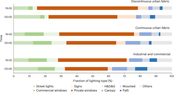
The bar graphs show the extrapolated fraction of lighting types in the early and late evening for the three land-cover types in turn. The three types of sign are combined, and ‘H&D&G’ stands for ‘house numbers, doorbells and garden decoration lights’.

The same subset of data (Germany only) was used to examine the additional parameters associated with the lights recorded by the citizen scientists (shielding, brightness and color). The vast majority of streetlights in Germany were either fully (48%) or partially (49%) shielded (Extended Data Fig. 4). Pathway lighting, which in general fulfills a similar visual objective as street lighting, was far more frequently unshielded (16%). The lack of shielding was even more common for lights mounted on the sides of buildings, where only 29% were fully shielded and 26% were unshielded. The majority (58%) of observed flood lights were unshielded, implying upward lighting rather than downward lighting. This practice was most common in continuous urban fabric areas, where 70% were unshielded.

The likelihood of a light source being described as bright or dim varied considerably depending on the light type (Supplementary Figs. 3 and 4) and to some extent on the geographical context (Extended Data Fig. 10). For example, house numbers were frequently reported as dim, but our participants told us during the campaign that they often appeared brighter in areas with little or no street lighting. This was reflected in the data, in that house numbers and doorbells were much more frequently reported as ‘bright’ in discontinuous than in continuous urban fabric. The color of lights varied considerably between light types (Extended Data Fig. 5), with canopy lights being reported as overwhelmingly (88%) white and streetlights the category most frequently classified as orange (46%). We also examined the frequency of use of presence detection for controlling at least one light on a transect (Extended Data Fig. 6). Currently, the use of motion control is more common in dimly lit villages and suburbs (29%) than in continuous urban fabric (15%) or industrial and commercial areas (11%).

The results provide a complete and large-scale lighting inventory of city lights and demonstrate the value of applying a citizen science approach to the problem of understanding lighting makeup on large spatial scales. Our participants classified all of the light sources visible over a walking distance of 600 km during an observation period of over 500 h. Whereas space-based sensors^17,25 can quickly survey large areas, they do not report what is actually installed on the ground (Fig. 1). In contrast, our application of human cognition provided a rich understanding of the types and properties of light sources. These results allow a ‘translation’ of satellite (DNB) radiance observations from radiometric units to lights per km², putting the scale of the problem of light pollution from cities into terms humans can relate to. For example, for DNB the number of lights in a German pixel can now be estimated simply by multiplying the average radiance (in nW cm⁻²sr⁻¹) first by 219 and then by the coverage area. If we assume that our observations are representative of the lighting practice in all of Germany, we estimate that on a typical clear night, the DNB observes the radiation emitted by approximately 2.52 ± 0.11 million individual light sources from Berlin and 78 ± 3 million light sources over the mainland of Germany (somewhat less than one light per person). This can be compared to a total estimate of 9–9.5 million public streetlights in Germany²⁶.

These results have implications for a number of application and research areas. For example, shielding lights to prevent upward emission is one of the most effective ways to prevent light pollution^11,27, but we found only about half of the German streetlight stock and 29% of lights mounted on buildings are fully shielded. Improving shielding is therefore an area that policymakers could focus on. The effectiveness of policy measures could be examined by a future lighting inventory. The results provide further evidence that it is not sufficient to consider only streetlights in studies of animal behavior²⁸ and simulations of skyglow¹². Within and near cities, skyglow studies have consistently observed radiance decreases^3,29,30,31 and color shifts^32,33 over the course of the night. These are both consistent with our observations of late-night extinction of residential and business lighting, underscoring the importance of including private lighting in research studies. This temporal change in city lighting also demonstrates the need for a more robust set of night-time light observations from space, particularly with regard to multiple overpass times¹⁷ and for remote sensing of human and economic parameters³⁴. This will be increasingly important with the transition to smart cities, where adaptive lighting emits light only when needed (Extended Data Fig. 6).

While we found correlations between the total number of light sources per square kilometer and satellite radiance, we were not able to estimate physically plausible weighting factors that reproduce the satellite datasets. Several factors may be responsible for this. First, Nachtlichter observations provide little radiometric information—in urban areas, signs with a luminance of 20 or 100 cd m⁻² would probably be classified as ‘normal’ but might both be classified as ‘bright’ in an area with little or no other light sources. Second, differences in building heights and street widths affect how easily light can escape to space³⁵. While a broad street may use the same number of streetlights as a narrow street, their overall lumen outputs are likely different. Indeed, our attempted algorithm often assigned a large (unphysical) weight to traffic lights, which are most often installed on wider, busier streets. In the future, Nachtlichter observations could be combined with information about urban morphology³⁶ and more detailed information about land use³⁷ to better estimate weighting factors. Nevertheless, our results already show that ground-based lighting inventories provide an important complement to satellite datasets and are probably necessary to understand the root causes of lighting change observed from space.

Ground-based surveys such as Nachtlichter could also help to explain geographical differences in urban light use. Countries with similar wealth and development often have dramatically (>200%) different average per capita light emissions observed from space^13,38. Even within a single country, emissions from cities with similar populations differ by up to an order of magnitude^27,38,39. It is still unclear why this is the case and to what extent it is due to differences in luminance⁴⁰ or types of light. A Nachtlichter-style approach could be used to obtain targeted observations in cities for which the satellite has identified a dramatic difference in total light emissions. The results of such a study could provide important information for sustainability science by identifying what industries, specific lighting applications or policy approaches are responsible for the differences. Furthermore, Nachtlichter observations could be used to assess the efficacy of lighting policy^{9,41,42,43,44,45}.

Street lighting has been the dominant focus of urban energy and environmental policy related to light⁴⁴. This is understandable as governments control these lights and they are an important contributor to total light emissions. Our data, however, confirm the finding that streetlights represent a minority of total light emissions from cities. The consequence of this narrow policy focus is illustrated by recent trends in skyglow radiance in the United States. In 2017, a Department of Energy report suggested that widespread conversion to light emitting diode (LED) street lighting was likely to decrease skyglow⁴⁶. However, observations of skyglow taken during 2011–2022, when many lights were converted, suggest a rapid (10% per year) increase¹⁵. While it is an open question as to whether existing approaches have failed to control the growth in emissions due to the neglect of private lighting or other factors, it is at least clear that existing policy results in increasing light growth.

New approaches to sustainable lighting policy that go beyond energy efficiency are therefore needed. For example, lighting regulation in France now requires advertising lighting to be turned off at hours when pedestrians are unlikely to be present and interior lights to be turned off when buildings are not occupied⁴⁷. This approach has the potential to reduce light emissions without adversely affecting advertisers. Matching streetlight provision to resident needs with lighting curfews⁴⁸ or motion sensors similarly reduces light without affecting objective or perceptive safety⁴⁹. Finally, because private windows are the most common outdoor light source, policy encouraging the use of curtains after sunset could have a larger impact than one might first assume.

The effectiveness of policy changes, for example, the degree of compliance among advertisers, could be tested in the future using the Nachtlichter methodology. In addition to providing an evidence-based assessment, this would have the advantage of increasing citizen participation in the evaluation and planning of city spaces. This may lead to further opportunities for energy and light savings as observations could help identify installations where light is being wasted. For example, our participants reported that 24% of bollards were bright, indicating that they were glaring or otherwise not well matched to the surroundings. In commercial and industrial areas, over a quarter of signs were reported as being exceptionally bright, which is consistent with previous research that has found that signs are often much brighter than is recommended or appropriate⁵⁰. This may reflect a need to update regulations about glare as the existing guidelines predate the use of highly luminous LEDs by several decades. Finally, we believe the involvement of citizens raises overall awareness of both effective and problematic lighting practice, as many of our participants have shared their insights with city leaders and in public presentations.

Limitations of the Nachtlichter methodology itself are discussed in Gokus et al.⁵, but some additional points apply to these analyses. The relation between DNB radiance and lights per km² appears to be specific to Germany and should be investigated in other countries before being applied. Areas with skyscrapers and private industrial parks were not surveyed and would need a different approach. The dimming or turning off of streetlights that occurs in many smaller German communities is not well captured here because of our lack of radiometric observations, the generally early time at which participants conducted their surveys and our limited number of observations from such communities. Finally, the contribution of car headlights remains unknown.

The Nachtlichter methodology has provided a unique measure of the status quo of lighting practice and its relation to upward radiance and land-cover type. Running the experiment in targeted areas, especially in other countries, could reveal the causes behind the large per capita variation in light emissions between and within developed countries³⁸. This would require a considerable effort, however, as the training materials and app would need to be adapted to different languages, and a native language team would need to coordinate each national campaign. This may become more feasible as future satellites with higher spatial resolutions and sensitivities are developed¹⁷ because the survey areas would not need to be as large as was the case for this analysis. With higher-resolution imagery, a targeted mix of transects with different characteristics (for example, urban, rural, commercial, industrial) could allow improved generalization of the results and modeling of light pollution and its impacts. Additionally, by repeating the experiment on the same transects after several years have passed, lighting change at the individual light source level could be studied. Such an effort would probably be most successful in the context of a long-term campaign, with sufficient resources allocated to participant recruitment, training and retention.

The Nachtlichter app was developed within a project called Nachtlicht-BüHNE (Citizen-Helmholtz Network for research on night light phenomena)⁵, using a co-design process in which academic and citizen scientists met regularly over a several year period. Our co-design process, app methodology, site selection, systematic variability of the observations, data pre-processing and data structure have already been described in detail⁵. This section therefore briefly covers the data and validation and focuses mainly on the methods unique to the analyses presented here.

Nachtlichter data and validation

In a Nachtlichter observation, participants conducted a ‘survey’ while walking along a ‘transect’, which typically extended from one street corner to the next. The participants used the app to classify and count all of the light sources that they could see. A total of 18 light categories were used for the 2021 experiment (Fig. 2). Depending on the light type selected, participants provided additional information about the size, emission direction (that is, shielding), color and subjective brightness. Transects were pre-defined in most cases and selected and arranged to completely survey the publicly accessible areas covered by a reprojected DNB satellite pixel. We therefore somewhat undercount the total number of installed lights because we did not record lights installed in areas not visible from public spaces (for example, backyards, courtyards and rooftops; Supplementary Fig. 5).

The observation time (of night) was not constrained, but the main experiment took place from 23 August to 14 November 2021, usually over a period of weeks for each pixel⁵¹. Additional smaller data-taking campaigns were conducted in the spring and autumn of 2022 to develop a correction for certain lighting types that were found to frequently turn off. The campaign in autumn of 2022 took place immediately after a German law requiring switch offs of some signs was passed²². However, as our statistics were not sufficient to observe a difference to the data taken in 2021, all of the available data were combined for determining the correction factors. The app and training materials were updated in 2023 to perform an experiment directly investigating lighting changes; data from that campaign is not included in the analyses reported here.

Observations were collected mainly in Germany from city centers, suburbs and villages (Extended Data Fig. 7). Region selection was based partly on where citizen scientists were present and able to count, and areas without sharp changes between land use near the boundaries were preferred⁵. Brighter areas in cities are therefore overrepresented compared to their relative frequency by area, but this means we cover nearly the full range of radiance observed for German communities¹³. Areas with high-rise buildings were generally avoided because of the difficulty in counting windows, but there were a few cases in which buildings of approximately ten stories were located along the transect. For most of the counting areas, buildings were one to four stories tall. The raw data may be downloaded from within the app itself (https://lichter.nachtlicht-buehne.de), and a processed dataset more suitable for analysis is available from GFZ Data Services⁵².

Observations were validated by comparing our total counts of streetlights to the numbers reported in public databases⁵. The values agreed to better than 7% for our areas in Berlin, Cologne and Dresden. In Fulda and Leipzig, the Nachtlichter counts were 40% and 90% larger, respectively. This was due to the presence of streetlights on private roads in these two measurement areas and exemplifies how Nachtlichter data are more complete than existing public lighting databases. Observations were additionally validated by comparing the counts of different participants to each other on the same transect. This was complicated by the fact that participants did not count at identical times, and later observations had fewer lights. The standard deviation for the total number of lights on the two most frequently observed streets was 15% for observations during 19:30–21:30. The counts were more consistent for streetlights than for other types of light, such as signs and windows, for which participants estimated sizes.

Time of night correction

As mentioned above, some light source types turn off during the course of the night⁵. Different satellite pixels were sampled at different dates of the campaign, and the earliest (by date) observations were acquired later at night, due to the late sunset. We therefore developed an approximate temporal correction to account for the changes and tested a few strategies using a Monte Carlo simulation of counting data. We found that the dataset size limitation would prevent fitting a general function. We therefore decided to model the switch off with a logistic function:

where p is the probability that a light is on at time t (in hours relative to midnight), f is the fraction of lights that turn off, s is a parameter that describes how quickly the lights turn off and h is the time (relative to midnight) at which half of the lights that will turn off have done so (Extended Data Fig. 8).

This function was motivated by published curves for private window illumination in Manhattan, New York, USA⁵³, and for its simple interpretation (for example, for private windows, h is effectively the average bedtime and s is related to the variability in bedtimes across the population). For most light source types, we do not have sufficient data to detect a change in lighting, or the returned fits did not describe the data well (for example, streetlights in Extended Data Fig. 8). For these sources, we do not apply a correction. The function is based on the assumption that all transects in Germany behave identically. While this is not the case, we found the fit for five of the light source types to be plausible and use it to extrapolate (or in some cases interpolate) the observations from each street to an estimate for what would have been observed at 19:00 and 00:00 (Extended Data Fig. 8 and Supplementary Table 1). The category ‘signs’ is based on the sum of illuminated signs, self-luminous signs and video screens. The same correction is applied to all three.

The fit parameters were found by minimizing the sum of errors over all surveys on transects with multiple observations. The individual survey error is defined by a least-squares-like function (Supplementary Fig. 6):

where N_c is the reported (counted) number of lights and N_e is the expected number of lights based on our fit. N_e is calculated via N_e(t) = N_t × p(t), where N_t is the estimated number of total lights on the transect in the early evening. N_t is found by minimizing E_surv for the current fit parameters. This minimization causes the red dots and yellow stars in Extended Data Fig. 8 to be distributed equally above and below the fit line as N_t is estimated separately for each transect.

The left term of equation (2) is similar to the usual weighted least-squares term for normally distributed data, but we have effectively increased the standard deviation to account for participant counting errors and the (frequently) small number of lights counted. However, our errors are not actually normal (or Poisson) distributed; large differences can occur if a set of lights is controlled by the same switch and turned off in unison, if a participant makes a dramatic counting error, or if the lights on the transect do not behave like the ‘average German street’. The right-hand term, therefore, minimizes the contribution of information from transects that do not behave in a typical fashion (that is, the difference compared to what we expected is larger than 3σ). In our tests based on Monte Carlo data, this procedure successfully returned fit parameters that reasonably match the inputs used in the simulation, even when we included the possibility of counting errors and correlated lights.

When a single Nachtlichter observation was made for a transect, the extrapolation process to obtain an estimate of the number of lights at an alternative time is straightforward. If N_c lights were observed (counted) at time t₀, then the estimated (maximum) total number of lights that would be turned on in the early evening for this transect is N_t = N_c/ p(t₀). The number of lights we would expect to be observed at a different given time t is then N_e = N_t × p(t). When a transect was surveyed multiple times, then N_t is estimated by finding the value of N_t that minimizes the sum of E_surv for all observations on the transect. The estimate at a given time t is then N_e = N_t × p(t) as before. For the light types for which no corrections are applied, multiple observations were simply averaged. These procedures lead to fractional values for the total number of lights.

Satellite data

The DNB⁵⁴ observes the Earth nightly at an equatorial crossing time of 1:30, with a consistent resolution of 750 meters across the scan. The detector is sensitive to electromagnetic radiation in the wavelength range 500 nm to 900 nm (for convenience referred to here as ‘light’). The combined light emissions from all sources within the ~0.56 km² is integrated into a single observed radiance value for the pixel. The nightly observations are combined into monthly and annual composite products by the Earth Observation Group²⁵, which uses a 15-arcsecond global raster. The pixel size therefore depends on latitude and is roughly 470 by 300 meters in central Germany (Fig. 1). Because the reprojected pixel is smaller than the intrinsic resolution, the radiance reported for a single pixel includes light from surrounding pixels. To the greatest extent possible, we therefore aimed to have Nachtlichter study sites located in areas surrounded by areas of similar character⁵. Nevertheless, the satellite radiance is biased downwards for lit areas near the city limits, and the radiance observed by adjacent DNB pixels is correlated.

We estimated the radiance of the Nachtlichter study areas using DNB observations taken during September through November during 2019 to 2021 (September 2021 was excluded because of considerable areas of Germany with no data, due to stray light on the sensor). We also calculated the total radiance from the mainland of Germany using airglow corrected data^55,56 for the months of October and November of 2015–2023 (a longer time series was used to better estimate uncertainties). The standard deviation of the sum of Germany’s lights was 7%, and the standard error was 1.7%. For Berlin, these numbers were 9% and 2.0%, and for our selection of DNB pixels (below), 12% and 4%.

Satellite and total lights analyses

We defined 181 analysis areas, usually associated with single DNB pixels (Fig. 1). In 12 cases, we joined multiple DNB pixels and Nachtlichter counts into a combined analysis area, as we felt it was more appropriate based on the relative positioning of the transects and pixel boundaries (for example, in the case of a single very long rural street segment that runs through multiple pixels and that was created directly by a participant rather than pre-defined by the main team). These were mainly in rural sites; the group of 12 had a median DNB radiance of 2.3 nW cm⁻²sr⁻¹.

We calculated the fraction of each transect that lay inside of a pixel boundary and multiplied this by the individual light type counts to obtain an estimate of how many of the transect’s lights are located inside of the pixel. These results were then summed to obtain a total number of counted lights within the pixel. The median relationship for all 181 analysis areas was 317 counted lights per km² per nW cm⁻²sr⁻¹. This is shown as a straight line in Fig. 3, and similar medians are shown in Extended Data Figs. 1 and 2 and Supplementary Figs. 1 and 2.

Graphing the median relationship is useful for showing when light types do or do not have a proportional relationship to satellite radiance, but it means pixels are weighted equally, rather than by the number of counted lights. As an alternative that assigns equal weight to counted lights and radiance, we divided the sum of counted lights over all pixels by the sum of the product of radiance and area for each individual pixel. This effectively treats all of our observations as if they were one single contiguous analysis area. When done for the German pixels only, and for the estimated light counts at midnight, we find a conversion factor of 219 ± 11 (standard error) lights per km² per nW cm⁻²sr⁻¹ (Supplementary Table 1 provides other selections). This factor was then multiplied by the product of mean radiance and total area to obtain the estimated number of lights that would be observed if all of Germany or all of Berlin were sampled using our methodology at midnight.

The Spearman rank correlation coefficient was calculated for each of the individual light types separately (Extended Data Figs. 1 and 2). In all cases, the (two-sided) null hypothesis of no correlation between satellite radiance and light type was rejected. The null hypothesis was least strongly rejected for garden decoration lights (p < 0.04) and house numbers and doorbells (p < 0.0002).

Uncertainty estimation

The estimation of the number of lights on at midnight is affected by three sources of uncertainty: person-to-person variability in the number of lights counted, uncertainty on the fit to the time-of-night light extinction curve and the uncertainty on the ‘sum of light’ from the DNB (reported above). The uncertainty on person-to-person variability was estimated via Monte Carlo. In a series of simulations, the sum of lights count (N_c) of each participant was adjusted according to N_sim = N_c/ v, where ‘v’ is an individual variability factor randomly chosen from a normal distribution with a standard deviation of 15%. We then calculated N_total = ∑N for each simulation and measured a standard deviation of 2.1%.

The uncertainty on both the fit parameters and the total lights at midnight were estimated using bootstrap with replacement⁵⁷. Each survey with N > 1 observations was assigned a statistical weight of N − 1 (because one degree of freedom is used for each transect to estimate the total number of lights). A total of 1,000 replacement samples were then randomly assembled with an equivalent statistical weight to the full sample, and the extinction curve was fit for each light type for this sample. For the uncertainty on the fit parameters, we report the confidence interval covering the 15.715th to 84.285th percentile (corresponding to 1σ; Supplementary Table 3). For each bootstrap dataset and fit, we then calculated the sum of lights for the five fit light categories and its standard deviation. We find that the fit introduces a standard error of 3.2% for the estimate of the total lights (all 18 categories) at midnight (Supplementary Table 4). The three uncertainties were then added in quadrature to yield a total standard error of 4.1% for Germany and 4.3% for Berlin.

Land-cover analysis

Our land-cover analysis makes use of the most recent CORINE (Coordination of Information on the Environment) Land Cover (CLC) classification from 2018⁵⁸. The CLC includes 44 different types of land cover, but 94% of our transects were located in one of just three land-cover classes: continuous urban fabric (typically city or town centers, with >80% of the land surface covered by impermeable features), discontinuous urban fabric (built-up areas with 30 to 80% of the surface covered by impermeable features) and industrial and commercial areas (Extended Data Figs. 9 and 10). Only 2% of transects were associated with the next most frequent land-cover class: urban green areas. Because our observations were made primarily in cities, the ‘industrial and commercial’ areas within this analysis are mainly commercial areas.

The minimal mapping unit of CLC is 25 ha. Because our transects are rarely longer than 200 meters, they are typically entirely within a single CLC class. (A higher-resolution land-cover dataset, such as the Copernicus Urban Atlas, would introduce additional complications, because transects would be more frequently split between land-cover types. It would also not be available for our rural sites.) We calculated the midpoint of each transect and assigned the transect to the land-cover category at that point. We then summed the light counts for all of the selected transects within the land-cover type, using the 19:00 and 00:00 projection for the overall comparison (Fig. 4) and the actually counted data (using the mean in case of multiple surveys) for the examination of the shielding, color and brightness properties (Extended Data Figs. 4 and 5 and Supplementary Figs. 3 and 4). For our examination of the prevalence of motion control detection (Extended Data Fig. 6), we treat each transect separately and show the maximal value reported. This is because in the early evening, observers may not notice that lights are activated based on presence detection, due to the higher number of people present on the street.

Light contribution analysis

Light is additive, so each light source located within a radiometer’s pixel increases the overall radiance measured by the instrument for that pixel proportional to its flux at the sensor. We attempted to find ‘weighting factors’ that would return radiance estimates based on the lights counted on the ground:

Here L_pred is the predicted radiance observed for a given pixel, w_i is a weighting factor for one of the 370 combinations of light and associated characteristics (for example, ‘video screen, small, medium brightness, white’), C_i is the total number of lights of that type observed within the pixel and the sum is over all of the different individual light types counted within the pixel. The values of w_i can be estimated by minimizing the value of a cost function that depends on them, such as:

Because we observed fewer than 370 DNB pixels, it was necessary to reduce the number of parameters. By assuming four variables representing the contribution of different sizes, emission directions, colors and brightnesses are constant across all lighting types, the number of variables could be reduced to 22. We attempted such minimizations with DNB, SDGSat and aerial photography data, with several different cost functions (the value of 0.2 above was motivated by the observation that the standard deviation of pixels in monthly DNB data is proportional to its radiance²⁴). Regardless of what we tried, the procedure never returned physically meaningful results.

Reporting summary

Further information on research design is available in the Nature Portfolio Reporting Summary linked to this article.

The raw data are available from within the Nachtlichter app at https://lichter.nachtlicht-buehne.de. Processed data are available from GFZ Data Services at https://doi.org/10.5880/GFZ.1.4.2024.006.

The code is available from GFZ Data Services at https://doi.org/10.5880/GFZ.1.4.2024.006.

References

Author notes

1. Andreas Ruby

   Present address: GFZ Helmholtz Centre for Geosciences, Potsdam, Germany

2. Yiğit Öner Altıntaş

   Present address: European Centre for Medium-Range Weather Forecasts, Bonn, Germany

Authors and Affiliations

1. Institute of Geography, Ruhr University Bochum, Bochum, Germany

   Team Nachtlichter, Andreas Rienow, Arne Dröge-Rothaar, Christopher Conrad Maximillian Kyba, Johannes A. Schultz & Kilian Modersitzki

2. Remote Sensing and Geoinformatics, GFZ Helmholtz Centre for Geosciences, Potsdam, Germany

   Team Nachtlichter, Christopher Conrad Maximillian Kyba, Helga Ursula Kuechly, Nona Schulte-Römer & Yiğit Öner Altıntaş

3. Independent researcher, Preußisch Oldendorf, Germany

   Achim Tegeler & Thomas Kunzemann

4. Independent researcher, Dresden, Germany

   Aleksander Marz, Bettine von Heereman, Christian Brock, Georg Sulzer, Maria Zschorn & Sicco Bauer

5. Department of Physics and McDonnell Center for the Space Sciences, Washington University in St. Louis, St. Louis, MO, USA

   Andrea Gokus

6. Fachgruppe Dark Sky, Georgsmarienhütte, Germany

   Andreas Hänel

7. Department of Physical Geography, Trier University, Trier, Germany

   Andreas Ruby

8. Independent researcher, Potsdam, Germany

   Anja Glinka, Janina Mattern & Reinhart Binder

9. Independent researcher, Wetaskiwin, Canada

   Anna Marie Kyba & Russell Kyba

10. Independent researcher, Fulda, Germany

    Axel Schwiesow & Peter Stumpf

11. Independent researcher, Erlangen, Germany

    Benno Gillen, Gisela Anton & Sebastian Falkner

12. Independent researcher, Herzogenaurach, Germany

    Brita Kuechly

13. Independent researcher, Kutahya, Turkey

    Burhan Altıntaş & Hatice Altıntaş

14. Sternwarte Dresden-Goennsdorf e.V, Dresden, Germany

    Christian Brock, Georg Sulzer & Sicco Bauer

15. Independent researcher, Westport, Ireland

    Cormac McNally

16. Independent researcher, Bochum, Germany

    Daniel Fischer

17. Independent researcher, Bolzano, Italy

    Daniele Dell’Osbel

18. Museum of Nature South Tyrol, Bozen, Italy

    David Gruber

19. Independent researcher, Munich, Germany

    Eva Constanze Weiß

20. Untere Naturschutzbehörde Köln, Köln, Germany

    Florian Distelrath & Irina von Maravić

21. Paten der Nacht gGmbH, Rimsting, Germany

    Frank Vohla

22. Hasso Plattner Institut, Potsdam, Germany

    Friedrich Heine

23. University of Galway, Galway, Ireland

    Georgia MacMillan

24. Center for Astrophysics, Harvard and Smithsonian, Cambridge, UK

    Gilbert A. Esquerdo

25. Independent researcher, Erfurt, Germany

    Henning von Brandis

26. Umweltzentrum Fulda e.V., Fulda, Germany

    Isabell Charis Wuthenow & Michaela Leipold

27. Independent researcher, Berlin, Germany

    Jacob Koglin & René Curwy

28. University of Würzburg, Würzburg, Germany

    Jacqueline Degen

29. Zentrum für Nationales Hochleistungsrechnen Erlangen, Erlangen, Germany

    Johannes Veh

30. Regionales Rechenzentrum Erlangen, Erlangen, Germany

    Johannes Veh

31. Dark Sky Consulting, Tucson, AZ, USA

    John C. Barentine

32. Independent researcher, Leverkusen, Germany

    Jonas Schreibweis

33. Nicolaus-Copernicus-Planetarium, Nürnberg, Germany

    Katharina Leiter

34. Independent researcher, Bonn, Germany

    Lena Klein

35. Lehrstuhl für Data Science in Earth Observation, Technische Universität München, Munich, Germany

    Marcus Langejahn

36. Faculty of Science and Mathematics, University of Split, Split, Croatia

    Marijana Pavić

37. Umweltinstitut Leipzig e.V., Leipzig, Germany

    Maximilian Blaschke & Steffen Liese

38. Planetarium Südtirol, Karneid, Südtirol, Italy

    Maximilian Köcher

39. Trier University, Trier, Germany

    Melanie Brauchler

40. Fachbereich Geodäsie, Bochum University of Applied Sciences, Bochum, Germany

    Nathalie Küppers

41. Institut für Europäische Ethnologie, Humboldt-Universität zu Berlin, Berlin, Germany

    Nona Schulte-Römer

42. Helmholtz-Zentrum für Umweltforschung - UFZ, Leipzig, Germany

    Nona Schulte-Römer

43. Independent researcher, Düsseldorf, Germany

    Normän Naboulsi

44. Faculty of Science, University of Split, Split, Croatia

    Petra Bilela, Tamara Rom & Vita Tičinović

45. Sternenpark Rhön, Fulda, Germany

    Sabine Frank

46. European Organization for the Exploitation of Meteorological Satellites, Darmstadt, Germany

    Yiğit Öner Altıntaş

Consortia

Contributions

Conceptualization: A.H., C.C.M.K., D.F., H.U.K., N.S.-R. and S.F. Data curation: A.D.-R., C.C.M.K., J.D., J.M., S.F. and Y.O.A. Methodology: A.D.-R., A.Gokus, A.H., A.M.K., A.Ruby, B.A., B.K., C.C.M.K., C.M., D.F., D.G., E.C.W., F.D., G.M., G.S., H.A., H.v.B., H.U.K., I.C.W., I.v.M., J.K., J.S., J.C.B., J.S., J.V., K.L., M.Blaschke, M.Brauchler, M.Langejahn, M.Liepold, M.P., M.Z., N.K., N.N., N.S.-R., P.B., P.S., R.B., R.C., R.K., S.B., S.Frank, S.Falkner, S.L., T.K., T.R., V.T. and Y.O.A. Investigation: A.T., A.M., A.Gokus, A.H., A.Ruby, A.Glinka, A.M.K., A.S., B.G., B.v.H., B.K., B.A., C.B., C.C.M.K., C.M., D.F., D.D., D.G., E.C.W., F.D., F.V., F.H., G.S., G.M., G.A.E., G.A., H.A., H.U.K., H.v.B., I.C.W., I.v.M., J.K., J.D., J.M., J.A.S., J.V., J.C.B., J.S., K.L., K.M., L.K., M.Langejahn, M.Z., M.P., M.Blaschke, M.K., M.Brauchler, M.Liepold, N.K., N.S.-R., P.S., P.B., R.B., R.C., R.K., S.Frank, S.Falkner, S.B., S.L., T.R., T.K., V.T. and Y.O.A. Visualization: A.D.-R., C.C.M.K., G.S., Y.O.A. and J.S. Funding acquisition: A.Rienow, C.C.M.K., H.U.K. and N.S.-R. Project administration: C.C.M.K., H.U.K. and N.S.-R. Supervision: A.Rienow and C.C.M.K. Writing—original draft: all authors. Writing—review and editing: all authors

Corresponding author

Correspondence to Christopher Conrad Maximillian Kyba.

Competing interests

The authors declare the following competing interests: several of the co-authors are members of advocacy groups that work in the area of light pollution (for example, DarkSky International) or on general environmental issues (for example, NABU).

Peer review information

Nature Cities thanks Noam Levin, Chu-wing So and the other, anonymous, reviewer(s) for their contribution to the peer review of this work.

Open Access This article is licensed under a Creative Commons Attribution 4.0 International License, which permits use, sharing, adaptation, distribution and reproduction in any medium or format, as long as you give appropriate credit to the original author(s) and the source, provide a link to the Creative Commons licence, and indicate if changes were made. The images or other third party material in this article are included in the article’s Creative Commons licence, unless indicated otherwise in a credit line to the material. If material is not included in the article’s Creative Commons licence and your intended use is not permitted by statutory regulation or exceeds the permitted use, you will need to obtain permission directly from the copyright holder. To view a copy of this licence, visit http://creativecommons.org/licenses/by/4.0/.

Reprints and permissions

References

Jägerbrand, A. K. & Spoelstra, K. Effects of anthropogenic light on species and ecosystems. Science 380, 1125–1130 (2023).
Zielinska-Dabkowska, K. M., Schernhammer, E. S., Hanifin, J. P. & Brainard, G. C. Reducing nighttime light exposure in the urban environment to benefit human health and society. Science 380, 1130–1135 (2023).
Falchi, F. et al. The new world atlas of artificial night sky brightness. Sci. Adv. 2, e1600377–e1600377 (2016).
Bonney, R. et al. Citizen science: a developing tool for expanding science knowledge and scientific literacy. BioScience 59, 977–984 (2009).
Gokus, A. et al. The Nachtlichter App: a citizen science tool for documenting outdoor light sources in public spaces. Int. J. Sustain. Light. 25, 24–66 (2023).
Luginbuhl, C. B., Lockwood, G. W., Davis, D. R., Pick, K. & Selders, J. From the ground up I: light pollution sources in Flagstaff, Arizona. Publ. Astron. Soc. Pac. 121, 185–203 (2009).
Kyba, C. C. M. et al. Direct measurement of the contribution of street lighting to satellite observations of nighttime light emissions from urban areas. Light. Res. Technol. 53, 189–211 (2021).
Bará, S., Bao-Varela, C. & Lima, R. C. Quantitative evaluation of outdoor artificial light emissions using low Earth orbit radiometers. J. Quant. Spectrosc. Radiat. Transf. 295, 108405 (2023).
Meier, J. in Urban Lighting, Light Pollution and Society (Routledge, 2014).
Papalambrou, A. et al. Planning an international dark-sky place in Aenos National Park, the first steps. IOP Conf. Ser.: Earth Environ. Sci. 899, 012039 (2021).
Cleaver, O. P. Control of Coastal Lighting in Anti-Submarine Warfare Report No. 746 (DTIC, 1943).
Simoneau, A. et al. Point spread functions for mapping artificial night sky luminance over large territories. Mon. Not. R. Astron. Soc. 504, 951–963 (2021).
Kyba, C. C. M. et al. Artificially lit surface of Earth at night increasing in radiance and extent. Sci. Adv. 3, e1701528 (2017).
Sánchez de Miguel, A., Bennie, J., Rosenfeld, E., Dzurjak, S. & Gaston, K. J. First estimation of global trends in nocturnal power emissions reveals acceleration of light pollution. Remote Sens. 13, 3311 (2021).
Kyba, C. C. M., Altıntaş, Y. Ö., Walker, C. E. & Newhouse, M. Citizen scientists report global rapid reductions in the visibility of stars from 2011 to 2022. Science 379, 265–268 (2023).
Bará, S. & Castro-Torres, J. J. Diverging evolution of light pollution indicators: can the globe at night and VIIRS-DNB measurements be reconciled? J. Quant. Spectrosc. Radiat. Transf. 335, 109378 (2025).
Linares Arroyo, H. et al. Monitoring, trends and impacts of light pollution. Nat. Rev. Earth Environ. 5, 417–430 (2024).
Rodriguez, A., Rodriguez, B. & Negro, J. J. GPS tracking for mapping seabird mortality induced by light pollution. Sci. Rep. 5, 10670 (2015).
Horton, K. G. et al. Artificial light at night is a top predictor of bird migration stopover density. Nat. Commun. 14, 7446 (2023).
Evens, R. et al. Skyglow relieves a crepuscular bird from visual constraints on being active. Sci. Total Environ. 900, 165760 (2023).
Bucher, S. F. et al. Artificial light at night decreases plant diversity and performance in experimental grassland communities. Philos. Trans. R. Soc. B 378, 20220358 (2023).
Bundesministerium der Justiz. EnSikuMaV - Verordnung Zur Sicherung Der Energieversorgung Über Kurzfristig Wirksame Maßnahmen, Bundesgesetzblatt (2022).
Kyba, C. et al. Methods and data of citizen science project Nachtlichter. GFZ Data Services https://doi.org/10.5880/GFZ.1.4.2023.002 (2023).
Coesfeld, J. et al. Variation of individual location radiance in VIIRS DNB monthly composite images. Remote Sens. 10, 1964 (2018).
Elvidge, C. D., Baugh, K., Zhizhin, M., Hsu, F. C. & Ghosh, T. VIIRS night-time lights. Int. J. Remote Sens. 38, 5860–5879 (2017).
Düsterdiek, B. et al. Öffentliche Beleuchtung Analyse, Potenziale und Beschaffung. https://www.dstgb.de/Publikationen/Dokumentationen/Nr.%2092%20-%20%C3%96ffentliche%20Beleuchtung%20-%20Analyse,%20Potentiale%20und%20Beschaffung/doku92.pdf?cid=6iv (2009).
Green, R. F., Luginbuhl, C. B., Wainscoat, R. J. & Duriscoe, D. The growing threat of light pollution to ground-based observatories. Astron. Astrophys. Rev. 30, 1 (2022).
Barré, K., Thomas, I., Le Viol, I., Spoelstra, K. & Kerbiriou, C. Manipulating spectra of artificial light affects movement patterns of bats along ecological corridors. Anim. Conserv. 26, 865–875 (2023).
Kyba, C. C. M. et al. Worldwide variations in artificial skyglow. Sci. Rep. 5, 8409 (2015).
Bará, S. et al. Estimating the relative contribution of streetlights, vehicles, and residential lighting to the urban night sky brightness. Light. Res. Technol. 51, 1092–1107 (2018).
Posch, T., Binder, F. & Puschnig, J. Systematic measurements of the night sky brightness at 26 locations in Eastern Austria. J. Quant. Spectrosc. Radiat. Transf. 211, 144–165 (2018).
Kyba, C. C. M., Ruhtz, T., Fischer, J. & Hölker, F. Red is the new black: how the colour of urban skyglow varies with cloud cover. Mon. Not. R. Astron. Soc. 425, 701–708 (2012).
Robles, J. et al. Evolution of brightness and color of the night sky in madrid. Remote Sens. 13, 1511 (2021).
Gibson, J., S, O. & G, B.-G. Night lights in economics: sources and uses. J. Econ. Surv. 34, 955–980 (2020).
Elvidge, C. D. et al. Indicators of electric power instability from satellite observed nighttime lights. Remote Sens. 12, 3194 (2020).
Espey, B. R., Yan, X. & Patrascu, K. Real-world urban light emission functions and quantitative comparison with spacecraft measurements. Remote Sens. 15, 2973 (2023).
Yan, G., Zou, L. & Liu, Y. The spatial pattern and influencing factors of china’s nighttime economy utilizing POI and remote sensing data. Appl. Sci. 14, 400 (2024).
Falchi, F. et al. Light pollution in USA and Europe: the good, the bad and the ugly. J. Environ. Manage. 248, 109227 (2019).
Kyba, C. C. M. et al. High-resolution imagery of Earth at night: new sources, opportunities and challenges. Remote Sens. 7, 1–23 (2015).
Levin, N. Quantifying the variability of ground light sources and their relationships with spaceborne observations of night lights using multidirectional and multispectral measurements. Sensors 23, 8237 (2023).
Aubé, M. & Roby, J. Sky brightness levels before and after the creation of the first international dark sky reserve, Mont-Mégantic Observatory, Québec, Canada. J. Quant. Spectrosc. Radiat. Transfer 139, 52–63 (2014).
Guanglei, W., Ngarambe, J. & Kim, G. A comparative study on current outdoor lighting policies in China and Korea: a step toward a sustainable nighttime environment. Sustainability 11, 3989 (2019).
Pérez Vega, C., Zielinska-Dabkowska, K. M., Schroer, S., Jechow, A. & Hölker, F. A systematic review for establishing relevant environmental parameters for urban lighting: translating research into practice. Sustainability 14, 1107 (2022).
Morgan-Taylor, M. Regulating light pollution: more than just the night sky. Science 380, 1118–1120 (2023).
Pothukuchi, K. Mitigating urban light pollution: a review of municipal regulations and implications for planners. J. Urban Aff. https://doi.org/10.1080/07352166.2023.2247506 (2023).
Kinzey, B. R. et al. An Investigation of LED Street Lighting’s Impact on Sky Glow Report No. PNNL-26411 (PNNL, 2017).
Arrêté Du 27 Décembre 2018 Relatif à La Prévention, à La Réduction et à La Limitation Des Nuisances Lumineuses (French Ministry of Ecology Sustainable Development and Energy, 2018).
Hessisches Netzwerk gegen Lichtverschmutzung. Nachtabschaltung https://www.lichtverschmutzung-hessen.de/Nachtabschaltung (2025).
Steinbach, R. et al. The effect of reduced street lighting on road casualties and crime in England and Wales: controlled interrupted time series analysis. J. Epidemiol. Commun. Health 69, 1118–1124 (2015).
Zielinska-Dabkowska, K. M. & Xavia, K. Global approaches to reduce light pollution from media architecture and non-static, self-luminous LED displays for mixed-use urban developments. Sustainability 11, 3446 (2019).
Zschorn, M. & Mattern, J. Counting lights for sustainability—insights from the citizen science project Nachtlicht-BüHNE. In Proc. Austrian Citizen Science Conference (eds Dörler, D. et al.) (PoS, 2022).
Dröge-Rothaar, A., Kyba, C. C. M., Falkner, S. & Altıntaş, Y. Ö. Nachtlichter 2021 campaign analysis software. GFZ Data Services https://doi.org/10.5880/GFZ.1.4.2024.006 (2025).
Dobler, G. et al. Dynamics of the urban lightscape. Inf. Syst. 54, 115–126 (2015).
Miller, S. et al. Illuminating the capabilities of the Suomi National Polar-Orbiting Partnership (NPP) Visible Infrared Imaging Radiometer Suite (VIIRS) day/night band. Remote Sens. 5, 6717–6766 (2013).
Stare, J. & Kyba, C. Radiance light trends. GFZ Data Services https://doi.org/10.5880/GFZ.1.4.2019.001 (2019).
Coesfeld, J., Kuester, T., Kuechly, H. U. & Kyba, C. C. M. Reducing variability and removing natural light from nighttime satellite imagery: a case study using the VIIRS DNB. Sensors 20, 3287 (2020).
Efron, B. in Breakthroughs in Statistics (eds Kotz, S. & Johnson, N. L.) 569–593 (Springer, 1992).
CORINE land cover. EEA https://doi.org/10.2909/71c95a07-e296-44fc-b22b-415f42acfdf0 (2020).
Acknowledgements
We thank all of the project participants who contributed to the development of the project and also everyone who collected data. In particular, we thank the following people who contributed sufficient data to be included as co-authors according to our authorship criteria but requested to be acknowledged by name instead: A. Peschl, B. Binder, B. Thébaudeau, G. Lelle, H. Bertram, I. Lelle, L. Quast, L. Dever, M. Blesius, M. Purtzel, N. Jankowiak, R. Paiarola, S. Marburger, S. Lohse-Koch, S. Euler-Bertram and W. Tsai. We also thank F. Klan, who led our partner project within the larger Nachtlicht-BüHNE project and who contributed to the initial conceptualization of the project. Finally, we thank A.Z., B.H., B.L., B.L., C.H., C.S., D.M., F.B., F.D., F.L., F.L., G.H., J.P., J.G., J.V., M.W., S.S., T.B. and V.S. These people made important contributions to the project but were not able to be contacted regarding co-authorship or named acknowledgement. Funding: Helmholtz Association Initiative and Networking Fund grant CS-0003 (C.C.M.K.). Helmholtz Association Initiative and Networking Fund grant ERC-RA-0031 (C.C.M.K.). Horizon 2020 grant 689443 via project GEOEssential (C.C.M.K.). Bundesministerium für Bildung und Forschung grants 01BF2202A and 01BF2202C (C.C.M.K.). Bundesministerium für Bildung und Forschung Wissen der Vielen–Forschungspreis für Citizen Science (C.C.M.K.).
Funding
Open access funding provided by GFZ Helmholtz-Zentrum für Geoforschung.
Ethics declarations