.png)

Main
Although the other fundamental interactions—electromagnetism and the strong and weak forces—have been successfully married to quantum theory, the standard methods of quantization seem to fail for gravity9. This has motivated alternative approaches to the unification of gravity with quantum theory, including string theory, loop quantum gravity and proposals that gravity is not quantized at all but remains fundamentally classical10. A decisive factor in determining which route is correct has so far been lacking: experimental evidence. At the 1957 Chapel Hill conference, Feynman proposed a thought experiment that could reveal the quantum nature of gravity1, an idea now becoming feasible through rapid progress in quantum experiments5,6. In Feynman’s proposal, an object of Planck mass (0.02 mg) is placed in a quantum superposition of two locations before interacting gravitationally with another mass1. Although Feynman’s exact measurement prescription for then determining the quantum nature of gravity is unclear from the original conference transcript1, today this is considered as the observation of entanglement between the massive objects, with several theorems on how physically realistic (local) classical theories of gravity can never create entanglement between the massive objects2,3,4,5,6,7,8. These theorems rest on the assumption that theories of classical gravity can involve only local operations and exchanges of classical information2,3,4,5,6,7,8. This is because non-local, action-at-a-distance processes are considered unphysical, and it seems natural that a classical gravitational interaction cannot transmit quantum information. Under this assumption, the interaction falls into a class of processes that, according to quantum information theory or generalizations7,8, cannot create entanglement, formalized as local operations and classical communication (LOCC) in quantum information theory3,5.
A substantial number of experimental proposals have been developed for witnessing this gravitationally induced entanglement11,12,13, and initial work on such experiments is underway11,14,15,16,17. Owing to the fundamental significance of the experiments, several works have appeared on whether entanglement can really provide evidence for quantum gravity, which are often inspired by discussions at the Chapel Hill conference1. These works have focused on whether classical gravity can act through non-local operations violating the LO part of LOCC and, thus, whether classical gravity can generate entanglement through non-local means (for a review, see refs. 12,18 and Supplementary Information). However, this goes against our understanding of interactions in nature acting locally, whether they are based on electromagnetism, the Standard Model or general relativity, and is, thus, generally ruled out on physical grounds2,3,5,6,18,19.
Assuming the LO part of LOCC on physical grounds, leaves the CC part. The idea that a classical theory of gravity should involve only classical communication seems natural and has not been questioned. However, here we show that local classical theories of gravity can, in fact, generate quantum communication and, thus, entanglement. The arguments and theorems for classical gravity operating only as LOCC implicitly treat matter in standard quantum mechanics. However, to the best of our knowledge, matter obeys quantum field theory (QFT), and when this is taken into account, we show that a classical gravity interaction naturally gives rise to quantum communication.
Quantum electrodynamics
To better understand how classical gravity theories can generate quantum communication, we first review quantum electrodynamics (QED). This is our best theory for how matter interacts through electromagnetism, and it involves treating both matter and the electromagnetic field with QFT. The interaction Hamiltonian is
$${\widehat{H}}_{{\rm{int}}}^{{\rm{QED}}}=\int {{\rm{d}}}^{3}{\bf{x}}\,q{\widehat{A}}_{\mu }({\bf{x}})\widehat{\overline{\psi }}({\bf{x}}){\gamma }^{\mu }\widehat{\psi }({\bf{x}}),$$
(1)
where \(\widehat{\psi }({\bf{x}})\) is a charged fermionic field with q its charge, \(\widehat{\overline{\psi }}({\bf{x}})\) is the Dirac adjoint field, \({\widehat{A}}_{\mu }({\bf{x}})\) is the quantized 4-potential and γμ are the gamma matrices. Calculations with QED are mostly performed perturbatively, where we can intuitively view interactions through Feynman diagrams. For example, Fig. 1 (top left) describes an interaction between two electrons at first order in perturbation theory. In this diagram, the electromagnetic interaction between the electrons is mediated by a virtual photon, which can be viewed as quantum communication2,20.
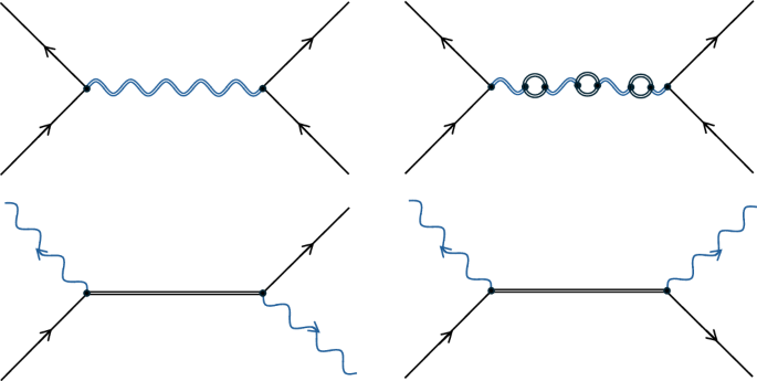
Wiggly blue lines represent photons or gravitons. Black lines represent electrons, positrons, or general matter or antimatter particles. For ease of visualization, double lines without arrows represent virtual particles.
However, a critical finding of QED compared with classical electromagnetism is that the interaction processes need not be mediated by just virtual photons. For example, at higher order in the electron-scattering process, there are diagrams such as Fig. 1 (top right) in which the virtual photon is accompanied by virtual electron particles. In fact, even at leading order there are processes that involve only virtual electron propagators, some of which are depicted in Fig. 1 (bottom row). When viewed from a non-perturbative perspective, there is no way to separate virtual matter from virtual photons in QED, and all electromagnetic interactions should be viewed as a combination of matter and electromagnetic fields propagating the interaction21.
Perturbative quantum gravity
Although there is no consensus on a full theory of quantum gravity, at low energies it is widely accepted that such a theory should approximate perturbative quantum gravity13,22,23,24,25. This is an effective field theory that involves the quantization of linear general relativity with matter fields: the full space-time metric gμν is broken up into ημν + hμν, with ημν the metric of a background classical space-time and ∣hμν∣ ≪ 1, which is quantized. The interaction Hamiltonian for matter interacting with gravity is
$${\widehat{H}}_{{\rm{int}}}^{{\rm{QG}}}=-\,\frac{1}{2}\int {{\rm{d}}}^{3}{\bf{x}}\,{\widehat{h}}^{\mu \nu }({\bf{x}}){\widehat{T}}_{\mu \nu }({\bf{x}}),$$
(2)
where \({\widehat{T}}_{\mu \nu }({\bf{x}})\) is the quantized energy–momentum tensor for matter. For example, describing matter with a massive complex scalar field \(\widehat{\phi }\), \({\widehat{T}}_{\mu \nu }({\bf{x}})\) becomes
$$\begin{array}{l}{\widehat{T}}_{\mu \nu }({\bf{x}})={\widehat{{\mathcal{T}}}}_{\mu \nu }[{\widehat{\phi }}^{\dagger }({\bf{x}})\widehat{\phi }({\bf{x}})]\\ \,\,:= \,{\partial }_{\{\mu }{\widehat{\phi }}^{\dagger }{\partial }_{\nu \}}\widehat{\phi }-{\eta }_{\mu \nu }{\partial }_{\rho }{\widehat{\phi }}^{\dagger }{\partial }^{\rho }\widehat{\phi }-{\eta }_{\mu \nu }\frac{{m}^{2}{c}^{2}}{{\hbar }^{2}}{\widehat{\phi }}^{\dagger }\widehat{\phi },\end{array}$$
(3)
where m is mass, c the speed of light and ħ the Planck constant. Here, \({\partial }_{\{\mu }A\,{\partial }_{\nu \}}B:= {\partial }_{\mu }A\,{\partial }_{\nu }B+{\partial }_{\nu }A\,{\partial }_{\mu }B\). The interaction Hamiltonian in equation (2) is of similar form to that in equation (1), and perturbative quantum gravity parallels QED closely18, with photons essentially being replaced with gravitons. For example, for two matter particles interacting, then at first order we have a diagram such as Fig. 1 (top left) but with a virtual graviton mediating the interaction rather than a virtual photon. Similarly, we also have all the other diagrams in Fig. 1, where there are virtual matter or virtual graviton propagators.
Perturbative classical gravity
In a fundamentally classical theory of gravity, the gravitational field is classical. Therefore, in the low-energy regime, most simply we would have an interaction Hamiltonian as equation (2) but with hμν not quantized:
$${\widehat{H}}_{{\rm{int}}}^{{\rm{CG}}}=-\,\frac{1}{2}\int {{\rm{d}}}^{3}{\bf{x}}\,{h}^{\mu \nu }(x)\,{\widehat{T}}_{\mu \nu }({\bf{x}}).$$
(4)
This is the interaction Hamiltonian of QFT in linear curved space-time, which, like any other QFT, is a local theory26,27,28.
The interaction Hamiltonian in equation (4) is analogous to that of an approximation sometimes performed in QED26,29,30,31: for certain QED calculations, such as Rutherford scattering, a good approximation is to ignore the quantumness of the electromagnetic field such that we drop the hat from Aμ in equation (1). Feynman diagrams can be drawn for this theory26, where a cross is often used to denote classical electromagnetic potentials and waves or, equivalently, a classical source for the electromagnetic field. For example, Fig. 2 (top left) illustrates an electron interacting with a classical potential or wave, and Fig. 2 (top middle) depicts how two electrons would interact in this theory, where now the cross can be seen as breaking quantum communication channels involving virtual photons in QED. However, certain diagrams still show virtual matter propagating the interactions, such as Fig. 2. (bottom row and top right).
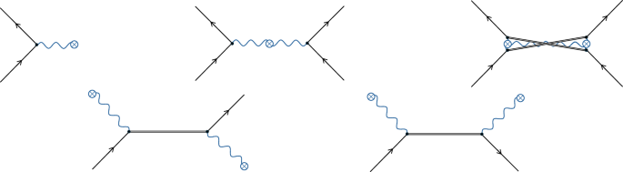
The wiggly blue lines are classical electromagnetic or gravitational fields or potentials. The crosses represent classical sources for the fields or potentials. As in Fig. 1, black lines represent electrons, positrons, or general matter or antimatter particles. For ease of visualization, double lines without arrows represent virtual particles.
Analogously, we can construct Feynman diagrams from the classical gravity interaction Hamiltonian in equation (4), where now wiggly lines with crosses in Fig. 2 denote classical gravitational potentials and waves. However, just as in the QED approximation, although there are no gravitons, there are still virtual matter propagators (see, for example, Fig. 2, bottom row and top right), and thus quantum communication. Then, as there is quantum communication, classical gravity can create entanglement2, violating the theorems and arguments discussed above4,5,6,7,8. This occurs because the theorems take a restrictive view on what the gravitational interaction consists of: they essentially assume that quantum gravity involves only virtual graviton propagators, but in fact, at the field theory level, there will also be virtual matter propagators.
Feynman’s experiment
To illustrate this further, we now demonstrate how equation (4) leads to entanglement in a version of Feynman’s experiment. Two spherical mass distributions, each with total mass M and radius R, are prepared in a quantum superposition of two locations. This could be achieved by, for example, implementing matter-wave beam splitters6, manipulating potentials32 or exploiting internal degrees of freedom, such as quantum spins in Stern–Gerlach experiments5 (Fig. 3). Gravity is assumed to be the only interaction between the particles, and in the non-relativistic limit and describing matter within first quantization, it just acts as a quantum phase φij ≔ GM2t/(ħ dij) on each superposition branch5,6, where dij is the distance between the matter distributions in the branch labelled by i, j ∈ {L, R}, and GM2/dij is the Newtonian potential energy. With the superposition size Δx much greater than the smallest distance dRL, only the quantum phase φ ≔ φRL is significant, so that the systems are clearly entangled, with the entanglement depending solely on φ (refs. 5,6). By contrast, when Δx ≪ dRL, the relevant parameter for entanglement becomes essentially \(\overline{\varphi }:= \varphi \,\Delta {x}^{2}/{d}_{{\rm{RL}}}^{2}\) (ref. 33). To measure the entanglement, the superposed paths could be recombined and correlations sought between the interferometer outputs6 or internal degrees of freedom5.
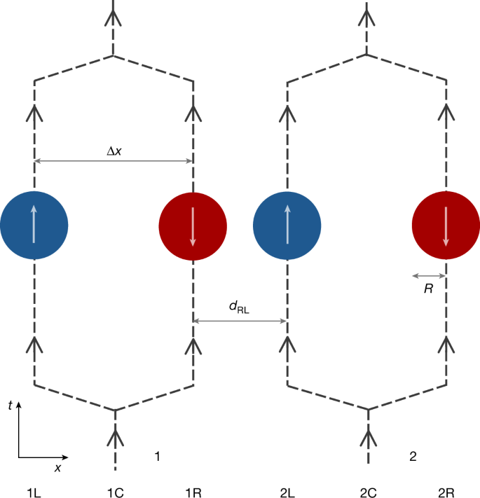
Two spherical mass distributions (1 and 2) of radius R are placed in quantum superpositions at two locations as N00N states, with blue and red denoting the components separated by Δx. After gravitationally interacting for a short time, the paths are recombined and entanglement is sought5,6. Although Stern–Gerlach interferometry with internal spins is illustrated5, alternative set-ups, such as parallel Mach–Zehnders, are also possible6. Here, Δx is depicted larger than the minimum separation dRL, but a general configuration can be implemented, including Δx ≪ dRL.
Quantum gravity
We now analyse this experiment using perturbative quantum gravity with a QFT description of matter. With electromagnetic interactions ignored, we take the initial state of the objects immediately after being placed in a quantum superposition as a product of N00N states:
$$\begin{array}{l}|\varPsi \rangle =\frac{1}{2}({|N\rangle }_{{\rm{1L}}}{|0\rangle }_{{\rm{1R}}}{|\uparrow \rangle }_{1}+{|0\rangle }_{{\rm{1L}}}{|N\rangle }_{{\rm{1R}}}{|\downarrow \rangle }_{1})\\ \qquad \otimes ({|N\rangle }_{{\rm{2L}}}{|0\rangle }_{{\rm{2R}}}{|\uparrow \rangle }_{2}+{|0\rangle }_{{\rm{2L}}}{|N\rangle }_{{\rm{2R}}}{|\downarrow \rangle }_{2}),\end{array}$$
(5)
where |N⟩κi is a product of N independent position states of matter particles obeying a complex scalar field34, with κ ∈ {1, 2} and i ∈ {L, R} labelling the position of the spherical objects (matching Fig. 3). N is the number of particles in the objects, such that M = mN, with m the mass of the particles. We also include possible internal spin states {|↑⟩, |↓⟩}, which could be used to generate the quantum superpositions.
After a time t, the state of the matter system in the Schrödinger picture is
$$| \varPsi (t)\rangle ={{\rm{e}}}^{{\rm{i}}{\widehat{H}}_{0}t/\hbar }\widehat{T}{{\rm{e}}}^{-({\rm{i}}/\hbar ){\int }_{0}^{t}{\rm{d}}\tau {\widehat{H}}_{{\rm{I}}}(\tau )}| \varPsi \rangle ,$$
(6)
where \(\widehat{T}\) is the time-ordering operator, τ is a dummy time variable, \({\widehat{H}}_{0}\) is the Hamiltonian of perturbative quantum gravity in the absence of matter–gravity interactions and \({\widehat{H}}_{{\rm{I}}}:= \exp ({\rm{i}}{\widehat{H}}_{0}t/\hbar ){\widehat{H}}_{{\rm{int}}}\,\exp (-{\rm{i}}{\widehat{H}}_{0}t/\hbar )\). Just before the superposition paths are bought back together, for example through reverse Stern–Gerlachs1,5, we can write
$$\begin{array}{l}|\,\varPsi (t)\rangle \propto {\alpha }_{{\rm{LL}}}{|N\rangle }_{{\rm{1L}}}{|N\rangle }_{{\rm{2L}}}+{\alpha }_{{\rm{LR}}}{|N\rangle }_{{\rm{1L}}}{|N\rangle }_{{\rm{2R}}}\\ \qquad \,+\,{\alpha }_{{\rm{RL}}}{|N\rangle }_{{\rm{1R}}}{|N\rangle }_{{\rm{2L}}}+{\alpha }_{{\rm{RR}}}{|N\rangle }_{{\rm{1R}}}{|N\rangle }_{{\rm{2R}}},\end{array}$$
(7)
where \({\alpha }_{ij}\in {\mathbb{C}}\). We have now neglected any internal spin states and the vacuum states for simplicity. We can calculate the amplitudes αij by taking the inner product of equation (7) (and also equation (6)), with the basis states |N⟩1i |N⟩2j and expanding the time-ordered unitary operation in equation (6) as the Dyson series26,35. The amplitudes can then be written as a perturbative series with each term corresponding to that of the Dyson series: \({\alpha }_{ij}={\alpha }_{ij}^{(0)}+{\alpha }_{ij}^{(1)}+{\alpha }_{ij}^{(2)}+\cdots \,\). The first process where a virtual graviton is exchanged between the matter objects occurs at second order in the series and corresponds to the Feynman diagram in Fig. 1 (top left). The amplitude for this Feynman diagram, within the very good approximation ct ≫ dij (Methods), is
$$\frac{G{M}^{2}t}{\hbar {V}^{2}}\iint {{\rm{d}}}^{3}{\bf{x}}\,{{\rm{d}}}^{3}{\bf{y}}\frac{{\theta }_{1i}({\bf{x}}){\theta }_{2j}({\bf{y}})}{| {\bf{x}}-{\bf{y}}| }\equiv {\varphi }_{ij},$$
(8)
where θκi(x) ≔ θ(R − ∣x − Xκi∣) is the unit-step function defining the spherical shape of the matter distribution κ in branch i, Xκi is the coordinate for the centre of mass for the distributions and V ≔ 4πR3/3. The above amplitude directly contributes to \({\alpha }_{ij}^{(2)}\) such that, when Δx ≫ dRL, the \({\alpha }_{{\rm{RL}}}^{(2)}\) amplitude dominates over all others and equals iφ. Then, given that \({\alpha }_{ij}^{(0)}=1\) from the Dyson series and that \({\alpha }_{ij}^{(1)}\) contains no contractions for the gravitational field, we are left with αij ≈ 1 except for αRL ≈ 1 + iφ, which matches the first-quantized result to first order in the quantum phase \(\exp ({\rm{i}}\varphi )\). The full non-perturbative result is straightforwardly obtained by considering the form of the corresponding higher-order Feynman diagrams and extrapolating the result26.
Classical gravity
We now consider the above experiment within the context of classical gravity. The calculation follows the above but with the interaction Hamiltonian of equation (4) rather than equation (2). At second order in the Dyson series there are no non-vanishing Wick contractions corresponding to Feynman diagrams that contain quantum communication between the matter objects, and the diagram responsible for entanglement in quantum gravity, Fig. 1 (top left), becomes Fig. 2 (top middle). This diagram represents the two matter objects sitting in their combined classical gravitational field, with the amplitude just contributing a local relative quantum phase between the branches of each matter object, which does not lead to entanglement13. However, at fourth order in the series, a diagram appears where the matter distributions are connected quantum mechanically through virtual matter particles (Fig. 2, top right). Within the same approximations as in the quantum gravity case, the amplitude for the Feynman diagram is (Methods)
$${{\vartheta }}_{ij}:= \frac{{m}^{6}{t}^{2}{N}^{2}}{4{{\rm{\pi }}}^{2}{\hbar }^{6}{V}^{2}}{\left(i\int {{\rm{d}}}^{3}{\bf{x}}{{\rm{d}}}^{3}{\bf{y}}\frac{\varPhi ({\bf{x}})\varPhi ({\bf{y}}){\theta }_{1i}({\bf{x}}){\theta }_{2j}({\bf{y}})}{| {\bf{x}}-{\bf{y}}| }\right)}^{2},$$
(9)
where Φ(x) ≔ −c2h00(x)/2 is the total gravitational potential of the matter objects, and ϑij directly contributes to \({\alpha }_{ij}^{(4)}\) in equation (7). As we have a classical theory of gravity, Φ(x) is the same in each superposition branch, otherwise the Newtonian force would be in a quantum superposition. Certain works have considered gravity to be classical but still allow the field or Newtonian force to be in a quantum superposition36,37,38,39. Here, we keep to the notion that quantum superposition is a purely quantum-mechanical phenomena such that Φ(x) is not superposed in equation (9) and is not a quantum operator. However, despite this, equation (9) generically results in entanglement, as θ1i(x) and θ2i(x) are different for the different superposition paths and are connected through ∣x − y∣, such that \({\alpha }_{ij}^{(4)}\) is different for each superposition path, except for \({\alpha }_{{\rm{LL}}}^{(4)}={\alpha }_{{\rm{RR}}}^{(4)}\) from symmetry. We can understand this from the Feynman diagram in Fig. 2 (top right), where, unlike the gravitational potential, the virtual matter particles enter into a quantum superposition with the different mass states and the distance the virtual matter particles propagate is different in each branch, resulting in the spatial integrals in equation (9) being connected through ∣x − y∣.
As Φ(x) comes from a superposition of matter in equation (9), we must consider exactly how gravity is sourced by quantum matter in a fundamental theory of classical gravity. In the approach most considered40,41, Φ(x) in equation (9) is the sum of the average potentials of the superposition states of the two objects. In this case, ϑij is inversely proportional to dij such that, if Δx ≫ dRL, the RL amplitude dominates over all others and is ∣ϑRL∣ ≈ ϑ, where (Methods)
$$\sqrt{{\vartheta }}=\frac{6}{25}\frac{{G}^{2}{m}^{2}{M}^{3}Rt}{{\hbar }^{3}{d}_{{\rm{RL}}}}.$$
(10)
The state in equation (7) is then clearly entangled, because, just as in quantum gravity, αRL contains a contribution ϑ that is not in any of the other amplitudes αij. Furthermore, like quantum gravity33, the inverse scaling of ϑij with dij allows \(\overline{{\vartheta }}:= {\vartheta }\,\Delta {x}^{2}/{d}_{{\rm{RL}}}^{2}\) to be identified as the relevant parameter for entanglement when Δx ≪ dRL.
Discussion
The quantum gravity effect, characterized by φ, depends strongly on the mass and duration chosen for the experiment. A range of mass values and durations have been considered for Feynman’s experiment1,5,6,11,42,43, with the Planck mass, Mp ≈ 10−8 kg, thought to play a significant role1,32,44. For example, in ref. 5, relatively small masses are suggested, M ≈ 10−14 kg, at the expense of long coherence times t ≈ 2 s and large superpositions Δx ≈ 0.1 mm, and with dRL = 200 μm, such that quantum gravity would be an order of magnitude greater than residual electromagnetic interactions (alternatively, a conducting screen can be placed between the objects to eliminate electromagnetic interactions45). However, long coherence times present a significant experimental challenge due to expected decoherence mechanisms33. For instance, the source of decoherence that is thought to be the most dominant5, namely the scattering of molecules from an imperfect vacuum, requires extremely low pressures of 10−15 Pa for M = 10−14 kg and t = 2 s, which presents a formidable challenge5,32,33. The rate of decoherence from scattering scales linearly with pressure but as M2/3 with mass, which is far weaker than the mass scaling M2 of φ (ref. 33). Therefore, as it allows for much lower pressures, using larger masses and smaller times may be experimentally preferable33, which has been considered in equivalent tests6,46,47 with times such as 1 μs and masses ranging from 10−12 kg to 1 kg (refs. 1,6,11,33,42,43). Smaller superposition sizes have also been considered, as creating large Δx has proven experimentally challenging thus far33.
The comparative strength of the classical and quantum gravity effects calculated above also depends strongly on the mass and duration of the experiment. Figure 4 compares the classical and quantum gravity effects, φ and ϑ, for various durations and masses for the experiment described in section ‘Feynman’s experiment’ with ytterbium as the material5. For relatively small masses M ≈ 10−14 kg and long durations t ≈ 2 s, ϑ is substantially smaller than φ. However, with masses approaching the Planck mass and beyond, ϑ becomes large enough (ϑ ≈ 0.1) such that entanglement due to the classical gravity process is significant, even at short durations. Thus, the mere observation of entanglement at these values in the experiment described above cannot be taken as evidence of quantum gravity.
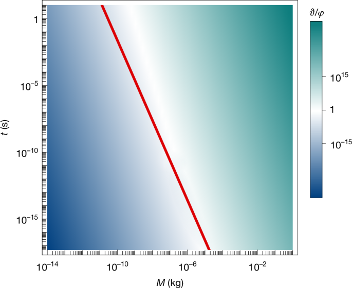
The relative strength of the considered effects ϑ/φ is shown for a range of masses M and times t in the experiment described in the main text. The red line and the region to the right of the line are where the classical gravity effect and its associated entanglement are significant (ϑ ≥ 0.1). To provide evidence of quantum gravity, the experiment must, therefore, operate to the left of this line. A minimum separation dRL = 10R is assumed, with R set by the total mass and density (note that ϑ is independent of the density) and m the mass of ytterbium. The ratio \(\overline{{\vartheta }}/\overline{\varphi }\), which characterizes the relative strength of the effects when dRL ≫ Δx, is identical to ϑ/φ.
The classical gravity process that is generating the entanglement is the exchange of virtual quantum matter associated with the gravitational interaction. Entanglement does not, thus, arise from just degrees of freedom that could be purely associated with the classical gravitational field5,6,7,8,48. As argued above, the very fact that gravity couples to matter implies, when quantum matter is treated within QFT, the possibility of having a matter propagator that can generate entanglement through the gravitational interaction, regardless of the specific form of the classical gravity model. Note that if, for example, electromagnetism were classical and we had electrically charged objects, then a similar equation to equation (9) could be derived with Φ(x) representing the Coulomb field of the objects. This could also, in principle, lead to entanglement, just as QED provides entanglement through an analogous expression to equation (8) through virtual photon exchange23,49. However, unlike with electromagnetism, we do not yet know if gravity is quantum. Here, we have shown that, although entanglement can be used to provide evidence for the quantum nature of gravity, contrary to that considered previously5,6,7,8, this is not unambiguous and is, instead, fundamentally a phenomenological issue: it depends on the parameters and form of the experiment.
Methods
The amplitude corresponding to the Feynman diagram in Fig. 1 (top left) can be computed by taking Wick contractions of the form
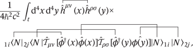
(11)
where 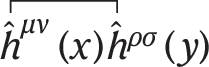 represents the Feynman graviton propagator \({\int }_{t}{{\rm{d}}}^{4}x:= \,\int {{\rm{d}}}^{3}{\bf{x}}{\int }_{0}^{ct}{\rm{d}}{x}^{0}\) and c is the speed of light. The above Wick contractions are evaluated using standard QFT techniques26, leading to equation (8) in the approximations of the experiment described in the main text and Fig. 3. A pedagogical overview of the calculations is provided in Supplementary Information.
The Feynman diagram in Fig. 2 (top right) corresponds to Wick contractions of the form
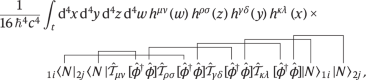
(12)
which is evaluated using standard QFT techniques26 and results in equation (9) in the approximations of the experiment described in the main text and Fig. 3. A full pedagogical derivation of how the above contraction leads to equation (9) is provided in Supplementary Information, where virtual matter processes in quantum gravity (which are always accompanied by graviton exchange) are also detailed.
As stated in the main text, Φ(x) in equation (9) is sourced by matter that is in a quantum superposition. The two leading suggestions for how this occurs in a fundamental theory of classical gravity are as follows: (1) Gravity is sourced by the mean expectation of matter \({\nabla }^{2}\varPhi ({\bf{x}})=\xi \langle {\widehat{T}}_{00}\rangle \) (refs. 40,41), where ξ = 4πG/c2, and the expectation is over the standard quantum state of matter or a generalization, such as a local description50,51,52. (2) Gravity is sourced by stochastic fluctuations around the mean expectation53,54,55,56: \({\nabla }^{2}\varPhi ({\bf{x}})=\xi [\langle {\widehat{T}}_{00}\rangle +\delta {T}_{00}]\), where δT00 is a stochastic quantity. The former has been studied more than the latter and is, thus, the option considered in the main text. A discussion on (2) is provided in Supplementary Information. The theoretical consistency of both cases has been debated, as also discussed in Supplementary Information, but neither has been ruled out experimentally. With option (1), Φ(x) in equation (9) is the sum of the average potentials of each mass distribution over their left and right states:
$$\varPhi ({\bf{x}})={\varPhi }_{{\rm{C1}}}({\bf{x}})+{\varPhi }_{{\rm{C2}}}({\bf{x}}),$$
(13)
with
$${\varPhi }_{{\rm{C}}\kappa }({\bf{x}}):= \frac{1}{2}({\varPhi }_{\kappa {\rm{L}}}({\bf{x}})+{\varPhi }_{\kappa {\rm{R}}}({\bf{x}})),$$
(14)
and
$$\begin{array}{c}{\varPhi }_{\kappa i}({\bf{x}}):= -\,GM\left[\left(\frac{3}{2R}-\frac{| {\bf{x}}-{{\bf{X}}}_{\kappa i}{| }^{2}}{2{R}^{3}}\right)\theta (R-| {\bf{x}}-{{\bf{X}}}_{\kappa i}| )\right.\\ \,\,\,\,+\left.\frac{\theta (| {\bf{x}}-{{\bf{X}}}_{\kappa i}| -R)}{| {\bf{x}}-{{\bf{X}}}_{\kappa i}| }\right],\end{array}$$
(15)
such that Φκi(x) is the gravitational potential of a spherical mass distribution of total mass M at position Xκi, and ΦCκ(x) is the average gravitational potential of spherical mass distributions each of mass M located at XκL and XκR. The above potential is then inserted into equation (9), and the amplitude can be computed using standard integration techniques, as demonstrated in Supplementary Information.
Data availability
There are no data to be shared.
Code availability
No generated code was central to the main results. However, Mathematica code used as a guide in calculations can be obtained upon request to the corresponding author.
References
Feynman, R. in The Role of Gravitation in Physics (eds DeWitt, C. M. & Rickles, D.) 250–256 (Edition Open Access, 1957).
Kafri, D. & Taylor, J. A noise inequality for classical forces. Preprint at https://arxiv.org/abs/1311.4558 (2013).
Kafri, D., Taylor, J. M. & Milburn, G. J. A classical channel model for gravitational decoherence. New J. Phys. 16, 065020 (2014).
Krisnanda, T., Zuppardo, M., Paternostro, M. & Paterek, T. Revealing non-classicality of inaccessible objects. Phys. Rev. Lett. 119, 120402 (2017).
Bose, S. et al. Spin entanglement witness for quantum gravity. Phys. Rev. Lett. 119, 240401 (2017).
Marletto, C. & Vedral, V. Gravitationally induced entanglement between two massive particles is sufficient evidence of quantum effects in gravity. Phys. Rev. Lett. 119, 240402 (2017).
Marletto, C. & Vedral, V. Witnessing nonclassicality beyond quantum theory. Phys. Rev. D 102, 086012 (2020).
Galley, T. D., Giacomini, F. & Selby, J. H. A no-go theorem on the nature of the gravitational field beyond quantum theory. Quantum 6, 779 (2022).
Rovelli, C. Notes for a brief history of quantum gravity. In Proc. The Ninth Marcel Grossmann Meeting 742–768 (World Scientific, 2002).
Carlip, S. Is quantum gravity necessary? Class. Quantum Gravity 25, 154010 (2008).
Bose, S. et al. Massive quantum systems as interfaces of quantum mechanics and gravity. Rev. Mod. Phys. 97, 015003 (2025).
Huggett, N., Linnemann, N. & Schneider, M. D. Quantum Gravity in a Laboratory? (Cambridge Univ. Press, 2023).
Carney, D., Stamp, P. C. E. & Taylor, J. M. Tabletop experiments for quantum gravity: a user’s manual. Class. Quantum Gravity 36, 034001 (2019).
Delić, U. et al. Cooling of a levitated nanoparticle to the motional quantum ground state. Science 367, 892–895 (2020).
Westphal, T., Hepach, H., Pfaff, J. & Aspelmeyer, M. Measurement of gravitational coupling between millimetre-sized masses. Nature 591, 225–228 (2021).
Panda, C. D. et al. Measuring gravitational attraction with a lattice atom interferometer. Nature 631, 515–520 (2024).
Margalit, Y. et al. Realization of a complete Stern-Gerlach interferometer: toward a test of quantum gravity. Sci. Adv. 7, 2879 (2021).
Christodoulou, M., Biagio, A. D., Howl, R. & Rovelli, C. Gravity entanglement, quantum reference systems, degrees of freedom. Class. Quantum Gravity 40, 047001 (2023).
Marletto, C. & Vedral, V. Answers to a few questions regarding the BMV experiment. Preprint at https://arxiv.org/abs/1907.08994 (2019).
Bose, S., Mazumdar, A., Schut, M. & Toroš, M. Mechanism for the quantum natured gravitons to entangle masses. Phys. Rev. D 105, 106028 (2022).
Cao, T. Y. (ed.) Conceptual Foundations of Quantum Field Theory (Cambridge Univ. Press, 1999).
Howl, R. et al. Non-Gaussianity as a signature of a quantum theory of gravity. PRX Quantum 2, 010325 (2021).
Christodoulou, M. et al. Locally mediated entanglement in linearized quantum gravity. Phys. Rev. Lett. 130, 100202 (2023).
Wallace, D. Quantum gravity at low energies. Stud. Hist. Philos. Sci. 94, 31–46 (2022).
Donoghue, J. Quantum gravity as a low energy effective field theory. Scholarpedia 12, 32997 (2017).
Peskin, M. E. & Schroeder, D. V. An Introduction to Quantum Field Theory (Addison-Wesley, 1995).
Di Biagio, A., Howl, R., Brukner, Č., Rovelli, C. & Christodoulou, M. Circuit locality from relativistic locality in scalar field mediated entanglement. Preprint at https://arxiv.org/abs/2305.05645 (2023).
Fewster, C. J. & Verch, R. in Advances in Algebraic Quantum Field Theory (eds Brunetti, R. et al.) 125–189 (Springer, 2015).
Weinberg, S. The Quantum Theory of Fields, Volume 1: Foundations, 1st edn (Cambridge Univ. Press, 1995).
Mandl, F. & Shaw, G. Quantum Field Theory, 2nd edn (Wiley, 2010).
Dereziński, J. Quantum fields with classical perturbations. J. Math. Phys. 55, 075201 (2014).
Howl, R., Penrose, R. & Fuentes, I. Exploring the unification of quantum theory and general relativity with a Bose-Einstein condensate. New J. Phys. 21, 043047 (2019).
Aspelmeyer, M. in From Quantum to Classical (ed. Kiefer, C.) 85–95 (Springer, 2022).
Pavšič, M. Localized states in quantum field theory. Adv. Appl. Clifford Algebr. 28, 89 (2018).
Dyson, F. J. The S matrix in quantum electrodynamics. Phys. Rev. 75, 1736–1755 (1949).
Anastopoulos, C. & Hu, B.-L. Comment on ‘A spin entanglement witness for quantum gravity’ and on ‘Gravitationally induced entanglement between two massive particles is sufficient evidence of quantum effects in gravity’. Preprint at https://arxiv.org/abs/1804.11315v1 (2018).
Anastopoulos, C., Lagouvardos, M. & Savvidou, K. Gravitational effects in macroscopic quantum systems: a first-principles analysis. Class. Quantum Gravity 38, 155012 (2021).
Martín-Martínez, E. & Perche, T. R. What gravity mediated entanglement can really tell us about quantum gravity. Phys. Rev. D 108, 101702 (2023).
Fragkos, V., Kopp, M. & Pikovski, I. On inference of quantization from gravitationally induced entanglement. AVS Quantum Sci. 4, 045601 (2022).
Rosenfeld, L. On quantization of fields. Nucl. Phys. 40, 353–356 (1963).
Møller, C. The energy-momentum complex in general relativity and related problems. In Proc. Les théories relativistes de la gravitation 15–29 (CNRS, 1962).
Krisnanda, T., Tham, G. Y., Paternostro, M. & Paterek, T. Observable quantum entanglement due to gravity. npj Quantum Inf. 6, 12 (2020).
Howl, R., Cooper, N. & Hackermüller, L. Gravitationally-induced entanglement in cold atoms. Preprint at https://arxiv.org/abs/2304.00734 (2023).
Christodoulou, M. & Rovelli, C. On the possibility of laboratory evidence for quantum superposition of geometries. Phys. Lett. B 792, 64–68 (2019).
Van De Kamp, T. W., Marshman, R. J., Bose, S. & Mazumdar, A. Quantum gravity witness via entanglement of masses: Casimir screening. Phys. Rev. A 102, 062807 (2020).
Pedernales, J. S. & Plenio, M. B. On the origin of force sensitivity in tests of quantum gravity with delocalised mechanical systems. Contemp. Phys. 64, 147–163 (2023).
Bengyat, O., Di Biagio, A., Aspelmeyer, M. & Christodoulou, M. Gravity-mediated entanglement between oscillators as quantum superposition of geometries. Phys. Rev. D 110, 056046 (2024).
Oppenheim, J. & Weller-Davies, Z. Covariant path integrals for quantum fields back-reacting on classical space-time. Preprint at https://arxiv.org/abs/2302.07283 (2023).
Qvarfort, S., Bose, S. & Serafini, A. Mesoscopic entanglement through central-potential interactions. J. Phys. B 53, 235501 (2020).
Kent, A. Simple refutation of the Eppley-Hannah argument. Class. Quantum Gravity 35, 245008 (2018).
Kent, A. Nonlinearity without superluminality. Phys. Rev. A 72, 012108 (2005).
Giulini, D., Großardt, A. & Schwartz, P. K. in Coupling Quantum Matter and Gravity (eds Pfeifer, C. & Lämmerzahl, C.) 491–550 (Springer, 2023).
Diósi, L. A universal master equation for the gravitational violation of quantum mechanics. Phys. Lett. A 120, 377–381 (1987).
Tilloy, A. & Diósi, L. Sourcing semiclassical gravity from spontaneously localized quantum matter. Phys. Rev. D 93, 024026 (2016).
Layton, I., Oppenheim, J., Russo, A. & Weller-Davies, Z. The weak field limit of quantum matter back-reacting on classical spacetime. J. High Energy Phys. 2023, 163 (2023).
Carney, D. & Matsumura, A. Classical-quantum scattering. Class. Quantum Gravity 42, 135010 (2025).
Acknowledgements
We both acknowledge support from the John Templeton Foundation as part of the QISS project (Grant No. 62312). R.H. also acknowledges Grant No. 62420 from the John Templeton Foundation. R.H. thanks members of the workshop ‘A look at the interface between gravity and quantum theory 2024’ for insightful discussions.
Ethics declarations
Competing interests
The authors declare no competing interests.
Peer review
Peer review information
Nature thanks Robert B. Mann and the other, anonymous, reviewer(s) for their contribution to the peer review of this work.
Additional information
Publisher’s note Springer Nature remains neutral with regard to jurisdictional claims in published maps and institutional affiliations.
Supplementary information
Rights and permissions
Open Access This article is licensed under a Creative Commons Attribution 4.0 International License, which permits use, sharing, adaptation, distribution and reproduction in any medium or format, as long as you give appropriate credit to the original author(s) and the source, provide a link to the Creative Commons licence, and indicate if changes were made. The images or other third party material in this article are included in the article’s Creative Commons licence, unless indicated otherwise in a credit line to the material. If material is not included in the article’s Creative Commons licence and your intended use is not permitted by statutory regulation or exceeds the permitted use, you will need to obtain permission directly from the copyright holder. To view a copy of this licence, visit http://creativecommons.org/licenses/by/4.0/.
About this article
Cite this article
Aziz, J., Howl, R. Classical theories of gravity produce entanglement. Nature 646, 813–817 (2025). https://doi.org/10.1038/s41586-025-09595-7
Received: 24 September 2024
Accepted: 05 September 2025
Published: 22 October 2025
Issue date: 23 October 2025
DOI: https://doi.org/10.1038/s41586-025-09595-7