Consistent Hashing

2 hours ago 1

This post is an introduction to consistent hashing, an algorithm for designing a hash table such that only a small portion of keys has to be recomputed when the table's size changes.

Motivating use case

Suppose we're designing a caching web proxy, but the expected storage demands are higher than what a single machine can handle. So we distribute the cache across multiple machines. How do we do that? Given a URL, how do we make sure that we can easily find out which server we should approach for a potentially cached version [1]?

An approach that immediately comes to mind is hashing. Let's calculate a numeric hash of the URL and distribute it evenly between N nodes (that's what we'll call the servers in this post):

hash := calculateHashFunction(url) nodeId := hash % N

This process works but turns out to have serious downsides in real-world applications.

The problem with the naive hashing approach

Consider our caching use case again; in a realistic application at "internet scale", one of the assumptions we made implicitly doesn't hold - the cache nodes are not static. New nodes are added to the system if the load is high (or if new machines come into service); existing nodes can crash or be taken offline for maintenance. In other words, the number N in our application is not a constant.

The problem may be apparent now; to demonstrate it directly, let's take an actual implementation of hashItem using Go's md5 package [2]:

// hashItem computes the slot an item hashes to, given a total number of slots. func hashItem(item string, nslots uint64) uint64 { digest := md5.Sum([]byte(item)) digestHigh := binary.BigEndian.Uint64(digest[8:16]) digestLow := binary.BigEndian.Uint64(digest[:8]) return (digestHigh | digestLow) % nslots }

The terminology is slightly adjusted:

Instead of url, we'll just refer to a generic item
"Slot" is a common concept in hash tables: our hashItem computes a slot number for an item, given the total number of available slots

Let's say we started with 32 slots, and we hashed the strings "hello", "consistent" and "marmot". We get these slots:

hello (n=32): 22 consistent (n=32): 14 marmot (n=32): 13

Now suppose that another node is added, and the total nslots grows to 33. Hashing our items again:

hello (n=33): 18 consistent (n=33): 25 marmot (n=33): 19

All the slots changed!

This is a significant problem with the naive hashing approach. Whenever nslots changes, we get completely different slots for pretty much any item. In a realistic application it means that whenever a new node joins or leaves our caching cluster, there will be a flood of cache misses on every query until the new cluster settles. And node changes sometimes occur at the most incovenient times; imagine that the load is spiking (maybe a site was mentioned in a high-profile news outlet, or there's a live event streaming) and new nodes are added to handle it. This isn't a great time to temporarily lose all caching!

Consistent hashing

The consistent hashing algorithm solves the problem in an elegant way. The key idea is to map both nodes and items onto an interval, and then an item belongs to a node closest to it. Concretely, we take the unit circle [3], and map nodes and items to angles on this circle. Here's an example that explains how this method works in more detail:

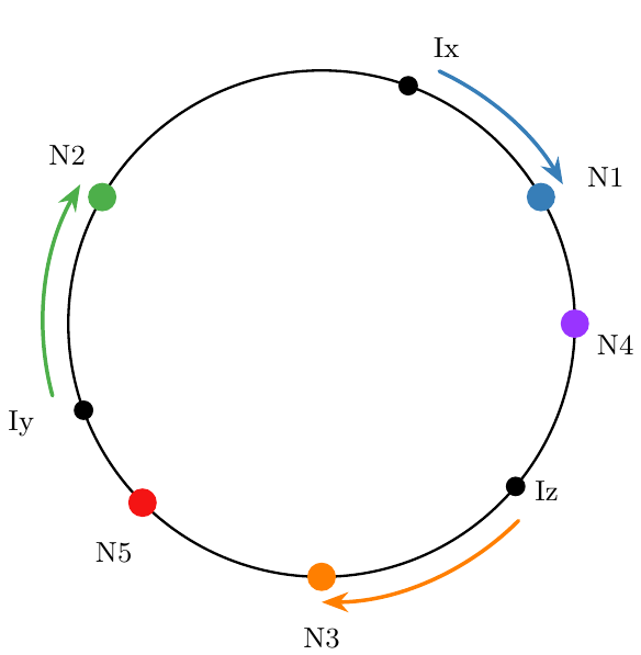
Circle showing consistent hashing in action

This shows five nodes: N1 through N5, and three items: Ix, Iy, Iz. Initially, we add the nodes: using a hashing operation we map them onto the circle (details later). Then, as items come in, we determine which node they belong to, as follows:

Use the same hashing operation to find the item's location on the circle
The node this item belongs to is the closest one, in the clockwise direction

In our diagram, Ix is mapped to N1, Iy to N2, and Iz to N3. So far so good, but the benefit of this approach becomes apparent when the nodes change. In our diagram, suppose N3 is removed. Then Iz will map to N5. The mapping of the other items doesn't change!

Adding nodes has a similar outcome. If a new node N6 is added and it hashes to a position between Iy and N2 on the circle, from that moment Iy will be mapped to N6, but the other items keep their mapping.

Suppose we have a total of M items that we need to distribute across N nodes. Using the naive hashing approach, whenever we add or remove a node, all M items change their mapping. On the other hand, with consistent hashing only about need to change. This is a huge difference.

The original consistent hashing paper (see [1]) calls this the monotonicity property of the algorithm:

If items are initially assigned to a set of buckets , and then some new buckets are added to form , then an item may move from an old bucket to a new bucket, but not from one old bucket to another.

Implementing consistent hashing

Implementing the consistent hashing algorithm as described above is fairly easy. The most critical part of the implementation is finding which node an item maps to - this involves some kind of search. The original consistent hashing paper suggests using a balanced binary tree for the search; the implementation I'm demonstrating here uses a slightly different but equivalent approach: binary search in a linear array of node positions (slots) [4].

First, some practical considerations:

Theoretically, the unit circle can be seen as the continuous range [0, 1). In programming we much prefer the discrete domain, however, so we're going to "quantize" this range to [0, ringSize), where ringSize is some suitably large number that avoids collisions.
Looking at the circle diagram above, imagine that 0 degrees is the "north" direction (12 o'clock), and angles increase clockwise. In our discrete domain, 12 o'clock is 0, 3 o'clock is ringSize/4, and so on.

When a node is added to the consistent hash, its location is found by applying a hash function like hashItem as described above, with nslots=ringSize. The nodes are stored using a pair of data structures, as follows; this example uses the approximate locations of the nodes N1 through N5 in the circle diagram above (assume ringSize=1024 here):

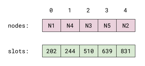
Nodes and slots arrays for the has shown above

The positions of the nodes on the circle are stored in slots, which is sorted. nodes holds the corresponding node names. For each i, nodes[i] is at position slots[i] on the circle.

Here's the ConsistentHasher data structure in Go:

type ConsistentHasher struct { // nodes is a list of nodes in the hash ring; it's sorted in the same order // as slots: for each i, the node at index slots[i] is nodes[i]. nodes []string // slots is a sorted slice of node indices. slots []uint64 ringSize uint64 } // NewConsistentHasher creates a new consistent hasher with a given maximal // ring size. func NewConsistentHasher(ringSize uint64) *ConsistentHasher { return &ConsistentHasher{ ringSize: ringSize, } }

And this is how finding which node a given item maps to is implemented:

// FindNodeFor finds the node an item hashes to. It's an error to call this // method if the hasher doesn't have any nodes. func (ch *ConsistentHasher) FindNodeFor(item string) string { if len(ch.nodes) == 0 { panic("FindNodeFor called when ConsistentHasher has no nodes") } ih := hashItem(item, ch.ringSize) // Since ch.slots is a sorted list of all the node indices for our nodes, a // binary search is what we need here. ih is mapped to the node that has the // same or the next larger node index. slices.BinarySearch does exactly this, // by returning the index where the value would be inserted. slotIndex, _ := slices.BinarySearch(ch.slots, ih) // When the returned index is len(slots), it means the search wrapped // around. if slotIndex == len(ch.slots) { slotIndex = 0 } return ch.nodes[slotIndex] }

The key here is the binary search invocation. Adding and removing nodes is done similarly using binary search - see the full code.

Better item distribution with virtual nodes

A common issue that comes up in the implementation of consistent hashing is unbalanced distribution of items across the different nodes. With items and a total of nodes, the average distribution will be about per node, but in practice it won't be very balanced - some nodes will have many more items assigned to them than others (see the Appendix for more details).

In a real application, this may mean that some cache servers will be much busier than others, which is a bad thing as far as capacity planning and efficient use of HW. Luckily, there's an elegant tweak to the consistent hashing algorithm that significantly mitigates the problem: virtual nodes.

Instead of mapping each node to a single location on the circle, we'll map it to V locations instead. There are several ways to do this - the simplest is just to tweak the node name in some way. For example, when AddNode is called to add node, it will run:

for i := range V { vnodeName = fmt.Sprintf("%v@%v", node, i) // ... now add vnodeName to the nodes/slots slices }

Then, when looking up an item we'll run into one of the virtual nodes, decode the node's name from it (in our example just strip the @<number> suffix) and return that. Implementing node removal is similarly simple.

The idea is that given a node named foo, the virtual node names foo@0, foo@1, foo@2 etc. will be spread all around the circle and not cluster in a single place. See the Appendix for a calculation of how this affects the final distribution.

The source code for this post includes a ConsistentHasherV type that is very similar to ConsistentHasher, except that it implements the virtual node strategy. The user interface remains exactly the same - it's only the internal implementation that changes slightly.

Code

The full source code for this post is on GitHub.

Appendix

The quality of the hash function is very important for good shuffling of nodes on the circle, but even if we take a perfect hash function that produces uniformly distributed values, the outcome is likely to be sub-optimal for our needs.

Let's say we select points on the unit circle, uniformly in the range [0, 1). If we sort the points by angle, the gaps between neighboring angles are the order statistics. These follow the Beta distribution with parameters (1, N-1), which has a mean of and a variance of .

This is quite significant. Consider a circle with 20 nodes. The standard deviation of the distribution is the square root of the variance; substituting , we get:

With 20 nodes uniformly distributed around a circle, we can expect an average of 18 degrees distance between two nodes. A standard deviation of 0.048 means 17 degrees, which is comparable to the average!

We can also do a realistic example to demonstrate this. Let's generate 20 random angles on a circle, and show how the node distribution looks:

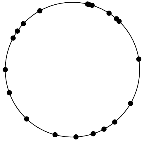
Circle with randomly distributed points

In this particular sample, the average angle between two adjacent nodes is 18 degrees (as expected). The smallest angle is just 1.04 degrees, while the largest one is 42 degrees. This means that some nodes will get 40x as many items assigned to them as others!

It's easy to see how virtual nodes help; imagine that each server maps to some number of randomly distributed nodes on the circle; some of these will be farther than others from their closest neighbor, but the average will have much less variety. Mathematically, given a set of n uniformly distributed random variables with variance v, the variance of their average is .

As a concrete experiment, I ran a similar simulation to the one above, but with 10 virtual nodes per node. We'll consider the total portion of the circle mapped to a node when it maps to either of its virtual nodes. While the average remains 18 degrees, the variance is reduced drastically - the smallest one is 11 degrees and the largest 26.

You can find the code for these experiments in the demo.go file of the source code repository.

Read Entire Article