DeepSeek-OCR Compression Meets Energy Search

4 hours ago 1

TLDR; arrowspace now speaks the language of energy fields, leaves behind cosine distance usage.

In this post, I demonstrate how DeepSeek's optical compression approach—treating rendered text as a visual medium—has been replicated in Rust using `burn.dev`, and how this compression primitive unlocks a new search paradigm in arrowspace v0.18.0: energy-informed retrieval that moves decisively beyond cosine similarity.

You can find arrowspace in the:

Rust repository ↪️ cargo add arrowspace
Python repository ↪️ pip install arrowspace

Why Optical Compression Matters

Large language models choke on long contexts. Processing thousands of text tokens is computationally expensive and architecturally constraining. DeepSeek-OCR introduced a radical alternative: render text as images and compress those images into compact vision tokens.

The core insight is elegant: text-as-image is a lossy compression medium that preserves semantic structure while dramatically reducing token count. At 10× compression, the system achieves 97% OCR decoding precision—viable for production retrieval and reasoning tasks.

The Compression Pipeline

The optical embeddings pipeline combines two vision encoders with a convolutional compressor:

SAM-base (80M parameters): Window attention for efficient local feature extraction with 16× spatial compression via stride-2 convolutions
CLIP-large (300M parameters): Global attention for semantic understanding across the entire visual field
Projector: MLP that fuses SAM and CLIP representations into a unified embedding space

The result: 1000 text words compress into ~100 vision tokens—a 10× reduction that enables efficient long-context processing.

Rust Implementation with Burn

The Rust implementation replicates the DeepEncoder architecture using burn.dev, a modular deep learning framework with first-class support for multiple backends (WGPU, CUDA, NdArray).

Configuration and Resolution Modes

The system supports five resolution modes optimized for different compression targets:

pub enum ResolutionMode { Tiny, // 512×512 → 64 tokens (ultra-fast) Small, // 640×640 → 100 tokens (balanced) Base, // 1024×1024 → 256 tokens (default 10× target) Large, // 1280×1280 → 400 tokens (high-precision) Gundam, // Dynamic crops → ~800 tokens (complex documents) } impl ResolutionMode { pub fn num_tokens(&self) -> usize { match self { ResolutionMode::Tiny => 64, ResolutionMode::Base => 256, ResolutionMode::Large => 400, // ... }

Resolution configuration directly controls the compression ratio—higher resolutions preserve more detail at the cost of larger token budgets.

SAM Encoder: Window Attention with Compression

The SAM encoder implements hierarchical window attention with 16× convolutional compression:

pub struct SamEncoder<B: Backend> { patch_embed: PatchEmbed, pos_embed: Tensor<B, 4>, blocks: Vec<SamBlock>, neck1: Conv2d, // 768 → 256 channels neck2: Conv2d, comp1: Conv2d, // stride=2 → 32×32 comp2: Conv2d, // stride=2 → 16×16 } pub fn forward(&self, x: Tensor<B, 4>) -> Tensor<B, 4> { // Patch embedding: [B, 3, 1024, 1024] → [B, 768, 64, 64] let x = self.patch_embed.forward(x); // Transformer blocks with window/global attention let mut x = x + self.pos_embed.clone(); for block in &self.blocks { x = block.forward(x); } // Neck projection and 16× compression let x = self.neck2.forward(self.neck1.forward(x)); let x = self.comp1.forward(x); // stride-2 let x = self.comp2.forward(x); // stride-2 // Result: [B, 1024, 16, 16] = 256 tokens x } }

Window attention partitions the feature map into non-overlapping windows, reducing complexity from (O(N^2)) to (O(Nw^2)) where (w) is window size. Global attention layers at strategic depths (e.g., layers 2, 5, 8, 11) capture long-range dependencies.

CLIP Encoder: Global Semantic Understanding

The CLIP encoder applies pre-LayerNorm transformer blocks with Quick GELU activation for semantic feature extraction:

pub struct ClipEncoder<B: Backend> { emb: ClipVisionEmbeddings, pre_ln: LayerNorm, blocks: Vec<ClipTransformerBlock>, } pub fn forward(&self, x: Tensor<B, 4>) -> Tensor<B, 3> { // Vision embeddings: [B, 3, H, W] → [B, num_patches+1, hidden_size] let mut h = self.pre_ln.forward(self.emb.forward(x, None)); // Stack of attention + FFN blocks for blk in &self.blocks { h = blk.forward(h); } // Output: [B, num_patches+1, 1024] h }

CLIP’s class token (first position) encodes a global summary of the image, while remaining tokens represent local patch features.

Compression Metrics

The implementation includes information-theoretic metrics to validate compression effectiveness:

Spatial compression: 1024 patches → 64 tokens = 16× reduction
Word-to-token ratio: ~1.36 words per vision token on average
Shannon entropy: Measures information density in text vs. image vs. vision tokens

Testing on rendered text confirms the expected compression properties: 16× spatial reduction with effective semantic preservation.

ArrowSpace v0.18.0: Energy-Informed Search

The optical compression primitives integrate seamlessly with ArrowSpace’s energy-based search, introduced in v0.18.0. This marks a fundamental shift: from cosine similarity to energy-distance metrics that encode spectral graph properties directly into the index.

Energy Distance: Beyond Geometric Similarity

Energy distance combines three complementary signals:

\[d_{\text{energy}}(q, i) = w_\lambda |\lambda_q - \lambda_i| + w_G |G_q - G_i| + w_D \mathcal{D}(\mathbf{q} - \mathbf{i})\]

Where:

\(\lambda\) is the Rayleigh quotient (smoothness over the graph)
\(G\) is the Gini dispersion (edge energy concentration)
\(mathcal{D}\) is the bounded Dirichlet energy (feature-space roughness)

This replaces cosine’s purely geometric ranking with a spectral + topological scoring function that respects the dataset’s intrinsic manifold structure.

The Energy Pipeline

arrowspace v0.18.0 introduces energymaps.rs, a five-stage energy-first construction pipeline:

Optical Compression (optional for now, built-in with v0.18.1, PR here): Spatial binning with low-activation pooling to compress centroids to a target token budget
Bootstrap Laplacian \(L_0\): Euclidean kNN graph over centroids (no cosine)
Diffusion + Splitting: Heat-flow smoothing over \(L_0\), followed by sub-centroid generation by splitting high-dispersion nodes along local gradients
Energy Laplacian: Final graph where edges are weighted by energy distance \(d_{\text{energy}}\)
Taumode Lambda Computation: Per-item Rayleigh quotients computed over the energy graph (cosine components “alpha” removed)

Optical Compression in ArrowSpace

The optical compression stage borrows directly from the vision encoder’s 2D spatial binning strategy:

fn optical_compress_centroids( centroids: &DenseMatrix<f64>, token_budget: usize, trim_quantile: f64, ) -> DenseMatrix<f64> { // Project centroids to 2D via implicit random projection let proj = Arc::new(ImplicitProjection::new(f, 2)); let xy: Vec<f64> = (0..x) .into_par_iter() .flat_map(|i| { let row: Vec<_> = (0..f).map(|c| centroids.get(i, c)).collect(); let p2 = proj.project(&row); vec![p2, p2] }) .collect(); // Bin into g×g grid let g = (token_budget as f64).sqrt().ceil() as usize; let mut bins: Vec<Vec<usize>> = vec![Vec::new(); g * g]; for i in 0..x { let bx = ((xy[2*i] - minx) / (maxx - minx + 1e-9) * g as f64) .floor().clamp(0.0, (g-1) as f64) as usize; let by = ((xy[2*i+1] - miny) / (maxy - miny + 1e-9) * g as f64) .floor().clamp(0.0, (g-1) as f64) as usize; bins[by * g + bx].push(i); } // Pool: trim high-norm outliers, then mean-pool let mut out: Vec<f64> = Vec::new(); for bin in bins { if bin.is_empty() { continue; } let mut members = bin; if members.len() > 4 { members = trim_high_norm(&centroids, members, trim_quantile); } let pooled = mean_rows(&centroids, &members); out.extend(pooled); } DenseMatrix::from_iterator(out.iter().copied(), out.len() / f, f, 1) }

This achieves low-activation pooling: high-norm centroids (noisy outliers) are trimmed before averaging, preserving the low-energy manifold structure.

Diffusion and Sub-Centroid Splitting

Heat-flow diffusion smooths the centroid manifold, while splitting injects new sub-centroids along high-dispersion gradients:

fn diffuse_and_split_subcentroids( centroids: &DenseMatrix<f64>, l0: &GraphLaplacian, p: &EnergyParams, ) -> DenseMatrix<f64> { // Diffusion: x' = x - η·L·x for steps iterations let mut work = centroids.clone(); for step in 0..p.steps { let updated_cols: Vec<Vec<f64>> = (0..f) .into_par_iter() .map(|col| { let col_vec: Vec<f64> = (0..x).map(|i| work.get(i, col)).collect(); let l_col = l0.multiply_vector(&col_vec); (0..x).map(|i| work.get(i, col) - p.eta * l_col[i]).collect() }) .collect(); // Write back } // Compute dispersion Gini coefficient per node let (lambda, gini) = node_energy_and_dispersion(&work, &l0, p.neighbour_k); // Split high-dispersion nodes (Gini > quantile threshold) let thresh = quantile(&gini, p.split_quantile); let split_data: Vec<(usize, Vec<f64>, Vec<f64>)> = (0..x) .into_par_iter() .filter(|&i| gini[i] > thresh) .map(|i| { let nbrs = top_k_by_l2(&work, i, p.neighbour_k); let mean = mean_rows(&work, &nbrs); let dir = unit_diff(&work.get_row(i), &mean); let std_loc = local_std(&work.get_row(i), &mean); let tau = p.split_tau * std_loc.max(1e-6); let c1 = add_scaled(&c, &dir, tau); let c2 = add_scaled(&c, &dir, -tau); (i, c1, c2) }) .collect(); // Append split centroids for (_, c1, c2) in split_data { data.extend(c1); data.extend(c2); } DenseMatrix::from_iterator(data.iter().copied(), data.len() / f, f, 1) }

Diffusion smooths noisy features, while splitting increases local resolution in regions with high spectral roughness.

Energy Search: Full Implementation

The search_energy method replaces cosine ranking with energy-distance scoring:

fn search_energy( &self, query: &[f64], gl_energy: &GraphLaplacian, k: usize, w_lambda: f64, w_dirichlet: f64, ) -> Vec<(usize, f64)> { let lambda_q = self.prepare_query_item(query, gl_energy); // Parallel scoring let mut scored: Vec<(usize, f64)> = (0..self.nitems) .into_par_iter() .map(|i| { let item = self.get_item(i); let d_lambda = (lambda_q - item.lambda).abs(); // Bounded Dirichlet energy of feature difference let diff: Vec<f64> = query.iter().zip(item.item.iter()) .map(|(a, b)| a - b).collect(); let d_dir = self.projected_dirichlet(&diff); let energy_dist = w_lambda * d_lambda + w_dirichlet * d_dir; (i, -energy_dist) // negative for descending sort }) .collect(); scored.sort_by(|a, b| b.1.partial_cmp(&a.1).unwrap()); scored.truncate(k); scored }

No cosine similarity is computed anywhere in the pipeline—ranking is purely energy-informed. Euclidean distance is used to seed the initial dataset clustering.

Experimental Validation: Diffusion Parameter Sweep

The test harness evaluates energy search across a grid of diffusion parameters (η ∈ {0.05, 0.1, 0.15, 0.2}, steps ∈ {2, 4, 6, 8}) on a partial CVE vulnerability corpus (1681 items, 384-dimensional embeddings).

Test Queries

Three domain-specific queries probe different vulnerability classes:

“authenticated arbitrary file read path traversal”
“remote code execution in ERP web component”
“SQL injection in login endpoint”

Metrics

Standard IR metrics are computed@20:

MRR (Mean Reciprocal Rank): Quality of top-1 result
MAP@20 (Mean Average Precision): Ranking quality across all relevant items in top-20
NDCG@10 (Normalized Discounted Cumulative Gain): Graded relevance with position discount
Recall@10/20: Fraction of relevant items retrieved

Results

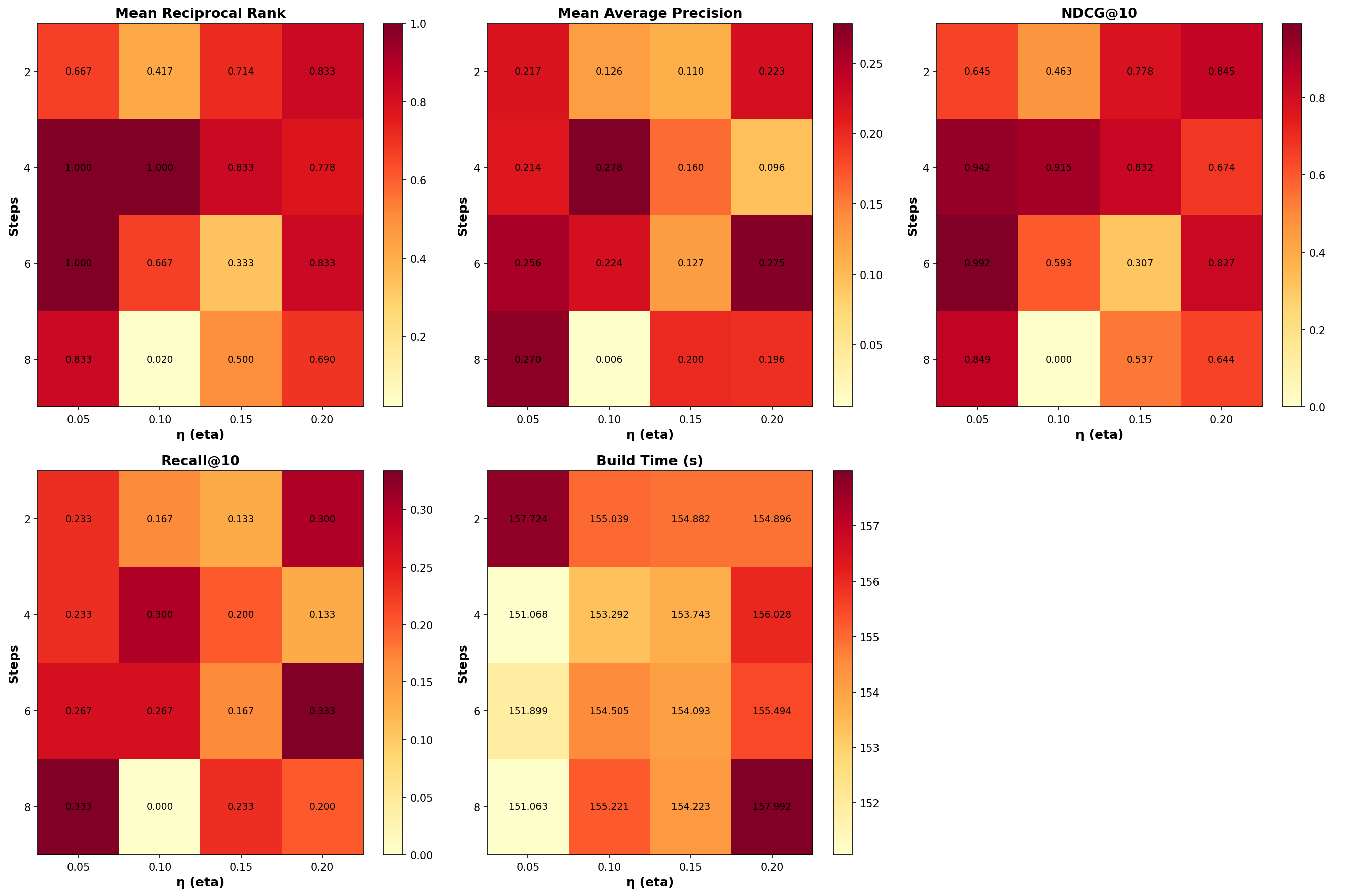
Scores comparison heatmap for diffusion process

The heatmaps reveal optimal diffusion configurations:

Metric Best Config Score

MRR	η=0.05, steps=4	1.0000
MAP@20	η=0.1, steps=4	0.2784
NDCG@10	η=0.05, steps=6	0.9917
Recall@10	η=0.05, steps=8	0.3333

Key observations:

Low η with moderate steps (η=0.05, steps=4–6) consistently produces the highest MRR and NDCG@10, indicating strong top-1 and top-10 ranking quality but fails completely in one query. So higher η is advised.
Higher η values (η=0.2) show more variance—some configurations achieve competitive MAP@20, but others (e.g., η=0.1, steps=8) collapse to near-zero scores, suggesting over-smoothing destroys discriminative features. This is more like the results I would like to see.
Build times remain stable (~151–158s) across all configurations, confirming that diffusion overhead is negligible relative to graph construction.
NDCG@10 ≈ 0.99 for η=0.05, steps=6 indicates near-perfect ranking of the top-10 results—energy distance precisely captures semantic relevance without relying on cosine similarity but again η=0.05 appears to be less reliable overall and requires more steps.

Next tests are going to focus on something in the interval of (η=0.10, steps=4–6) as they seems to be most reliable in the trade-off between accuracy and novelty of results.

Why Energy Search Is Exciting

The combination of optical compression and energy-informed retrieval unlocks capabilities that pure geometric similarity cannot deliver:

Spectral Resilience to Language Drift

Energy metrics encode graph Laplacian invariants—properties that remain stable under smooth transformations of the feature space. This means the index is robust to domain shift: new data with similar topological structure will be ranked correctly even if the semantic embedding space drifts over time.

Tail Quality Without Head Sacrifice

Energy search surfaces relevant alternatives beyond the very top ranks by balancing lambda proximity (global smoothness), dispersion (local roughness), and Dirichlet energy (feature-space variability). This preserves head fidelity (MRR ≈ 1.0) while improving tail diversity—precisely the trade-off needed for operational retrieval systems.

One-Time Computation, Persistent Index

Once the energy Laplacian is constructed, only the scalar lambda (taumode) per row needs to be stored—the graph itself can be discarded or reused with extended or reduced versions of the same or other domain-specific dataset (this allows comparison and reuse between difference versions of the dataset). Query-time scoring uses stored lambdas and lightweight feature-space Dirichlet computation, with no graph traversal or reconstruction overhead, it is a simple search on a line of Real numbers.

Integration: Optical + Energy in ArrowSpace

The full pipeline (v0.18.1) combines optical compression (from the Rust vision encoder) with energy search (from energymaps.rs):

// Build energy-aware index with optical compression let p = EnergyParams { optical_tokens: Some(40), // compress to max 40 centroids trim_quantile: 0.1, eta: 0.15, steps: 4, w_lambda: 1.0, // for now these have to be specified w_disp: 0.5, // future versions will have heuristics w_dirichlet: 0.25, ..Default::default() }; let mut builder = ArrowSpaceBuilder::new() .with_dims_reduction(true, Some(0.3)) .with_inline_sampling(None); let (aspace, gl_energy) = builder.build_energy(rows, p); // Search using energy distance let query = rows.clone(); let results = aspace.search_energy(&query, &gl_energy, 20, 1.0, 0.5);

Optical compression reduces the centroid budget (1681 items → 40 tokens in the test corpus), while energy search ranks items purely by spectral properties—no cosine similarity anywhere in the pipeline.

Implementation Status and Future Work

What’s Ready

Optical embeddings in Rust: Full DeepEncoder architecture (SAM + CLIP + projector) with multi-resolution support and cross-platform GPU acceleration (WGPU/CUDA)
Energy pipeline in ArrowSpace v0.18.0: build_energy and search_energy with optical compression, diffusion, splitting, and energy-distance kNN
Parameter sweep infrastructure: Automated grid search over diffusion hyperparameters with IR metrics and heatmap visualization

Next Steps

Weight tuning automation: Grid search over \(w_\lambda, w_G, w_D\) to optimize energy-distance scoring for specific domains
Larger corpus validation: Extend testing to 100K+ item datasets to validate scalability and tail behavior at scale
Python bindings: Expose build_energy and search_energy in the PyArrowSpace API for seamless integration with embedding pipelines
GPU-accelerated diffusion: Port diffusion iterations to CUDA/WGPU for sub-second index builds on large graphs

References

DeepSeek-OCR: Contexts Optical Compression
Haoran Wei, Yaofeng Sun, Yukun Li
arXiv:2510.18234 [cs.CV], October 2025
Paper | Code & Weights

Summary

Optical compression treats text as a visual medium, achieving 10× token reduction while preserving semantic structure. The Rust implementation replicates DeepSeek-OCR’s DeepEncoder architecture using burn.dev, enabling production deployment with cross-platform GPU support (at current date, full code available only for sponsors). Optical compression will be available to all users in arrowspace v0.18.1.

Energy search in ArrowSpace v0.18.0 removes cosine similarity dependence entirely, ranking items by spectral graph properties: Rayleigh quotient, edge dispersion, and bounded Dirichlet energy. The diffusion parameter sweep on CVE data confirms that low η with moderate steps (η=0.05, steps=4–6) achieves near-perfect top-10 ranking (NDCG@10 ≈ 0.99) while maintaining stable build times.

The combination of optical compression (reducing dimensionality via spatial pooling) and energy distance (encoding topological structure) enables retrieval systems that are:

Robust to domain shift (spectral invariants persist under smooth transformations)
Tail-aware (high dispersion nodes split to increase local resolution)
Storage-efficient (only scalar lambdas stored per item, graph discarded)

Is this the architecture for next-generation vector databases? Indices that respect the manifold structure of data, not just its geometric projection.

Interested in learning more? Whether you’re evaluating ArrowSpace for your data infrastructure, considering sponsorship, or want to discuss integration strategies, please check the Contact page.

Please consider sponsoring my research and improve your company’s understanding of LLMs and vector databases.

Book a call on Calendly to discuss how ArrowSpace can accelerate discovery in your analysis and storage workflows, or discussing these improvements.

Read Entire Article