Direct tensor processing with coherent light

Artificial intelligence technology, driven by neural networks, is rapidly reshaping various aspects of modern life. However, the training and inference processes of these networks impose enormous computational demands on digital processors. A key operation in these computations is tensor processing, typically implemented through matrix–matrix multiplication (MMM) on graphics processing unit (GPU) tensor cores^1,2,3,4. This approach, however, poses many challenges, including large memory bandwidth demands, substantial power consumption and inefficient use of tensor core resources. By contrast, optical computing, with its inherent characteristics of large bandwidth, high parallelism and low energy consumption, has emerged as a promising platform to compute and accelerate neural networks^5,6. State-of-the-art optical computing paradigms enable parallel dot product^7,8, vector–matrix multiplication^{9,10,11,12,13,14}, diffraction computing^15,16 and Fourier transform^17,18,19,20 by modulating the amplitude, phase and wavelength of light during a single propagation through planar waveguides or free space, laying the basis for various optical neural network (ONN) implementations^{21,22,23,24,25,26}.

While optical vector–matrix multiplication-driven ONNs are capable of executing tensor processing, they typically require multiple light propagations for each MMM operation, which limits their parallelism and overall efficiency. Some approaches have attempted to improve parallelism by leveraging space multiplexing^27,28, wavelength–time multiplexing^29,30, wavelength–space multiplexing^31,32,33,34 or precomputed inverse operations^21,35. However, these methods are constrained by device^28,36 and system design^29,37 and, in some cases, even contradict the fundamental principle of optical parallel acceleration at the computational logic level^38,39. By contrast, while diffraction-based computing offers high parallelism, it relies on diffraction principles to construct the computing architecture^40,41,42, making it unsuitable for general-purpose computation. As a result, existing optical computing paradigms struggle to balance both high parallelism and generality. They are often tailored to specific types of neural network computations or individual processing steps, rather than providing a universal acceleration framework for various complex neural network steps within a single system. This limitation also hinders the seamless deployment of advanced network models developed for GPUs onto optical computing platforms in the future.

Here, we report a direct parallel optical MMM (POMMM) paradigm for tensor processing that operates through a single coherent light propagation. This approach leverages the bosonic properties of light⁴³ and exploits the duality between the spatial position, phase gradients and spatial frequency distribution to enhance optical computing capabilities, adding an extra computational order without relying on additional time, space, wavelength multiplexing or preprocessing. We validate this paradigm through theoretical simulations and the construction of a physical optical prototype, demonstrating its strong consistency with standard GPU-based MMM over various input matrix scales. Building upon the POMMM simulation and prototype as fundamental computational units, we develop a GPU-compatible ONN framework and demonstrate the direct optical deployment of different GPU-based neural network architectures such as convolutional neural networks (CNNs)⁴⁴ and vision transformer (ViT) networks^45,46, incorporating various tensor operations such as multi-channel convolution, multi-head self-attention and multi-sample fully connected layers⁴⁷. We explored the scalability of POMMM, including its data type, large-scale computing ability for complex neural networks and tasks, and multi-wavelength multiplexing for high-order tensor processing. Finally, through a comprehensive comparison with existing optical computing paradigms, we highlight the superior performance of the POMMM paradigm as a transformative approach alongside the ONN framework it enables, offering theoretically improved efficiency and versatility in tensor processing. Our results demonstrate that POMMM has the potential to achieve more complex and higher-order general parallel optical computing, enabling future computing demands.

Conventionally, MMM between matrix A and matrix B is executed in two sequential steps. First, the Hadamard product (element-wise multiplication) is performed between each row of matrix A and each column of matrix B. Subsequently, the results of these Hadamard products are summed and assigned to their corresponding elements in the output matrix. Typically, the optical Hadamard product can be implemented by modulating the amplitude of spatial light, while the optical Fourier transform, which enables approximate summation or integration, can be achieved through quadratic phase modulation (for example, passing through a lens)⁴⁸. However, a key challenge remains: how to compute the dot products (sum after Hadamard product) of all rows of matrix A with all columns of matrix B (or all rows of matrix B^T, transpose of matrix B) in parallel and map them to their corresponding positions without mutual interference.

Fortunately, the Fourier transform exhibits two well-known properties: the time-shifting property and the frequency-shifting property. The former states that shifting a signal in the time (space) domain does not alter the amplitude distribution of its time (space) spectrum, while the latter indicates that applying a linear phase modulation in the time (space) domain results in a corresponding frequency shift in the time (space) spectrum. Leveraging these two properties, we construct the core concept of POMMM (Fig. 1a). First, the elements of matrix A are encoded onto the amplitude and position of a spatial optical field, with each row encoded by a linear phase with special gradient. Then, a column-wise Fourier transform is applied to the optical field carrying the complex amplitude signal, which can be implemented by imaging along the row direction and focusing along the column direction. At this stage, due to the time-shifting property, each row of the optical field represents the superposition of all rows of matrix A. Subsequently, amplitude modulation is applied to perform the Hadamard product between this ‘hybrid matrix’ and the matrix B^T, effectively enabling the parallel computation of all row-column Hadamard products. Finally, a row-wise Fourier transform is performed to complete the summation. Due to the frequency-shifting property and the presence of different linear phase modulations in the row dimension, the contributions from different rows of matrix A naturally separate into distinct spatial frequency positions in the final computational result (see details in Supplementary Note 1).

Fig. 1: Principle and experimental set-up of POMMM.

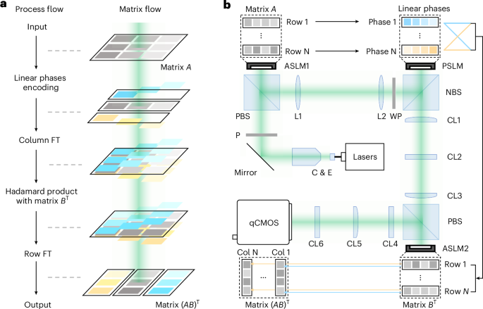
a, The operation principle of POMMM. Left: the process flow of POMMM. Right: the corresponding matrix process after each step. The different colours represent different linear phase encodings. FT, Fourier transform. b, Experimental set-up and corresponding matrix operations. C & E, collimation and expansion; P, polarizer; PBS, polarization beam splitter; L, lens; WP, wave plate; NBS, non-polarization beam splitter; qCMOS, quantitative complementary metal oxide semiconductor camera.

To experimentally validate POMMM using conventional optical components and demonstrate its functionality and compatibility, we design an optical proof-of-concept prototype (Fig. 1b). We first encode matrix A onto a collimated beam using an amplitude spatial light modulator (ASLM), ASLM1. This encoded beam is then imaged onto a phase spatial light modulator (PSLM) through a 4f optical system, where distinct linear phase modulations are applied to each row (these two steps can also be realized by a complex amplitude modulator). Subsequently, the beam passes through a cylindrical lens (CL) assembly (1, 2 and 3): two CLs (1 and 3) acting along the row direction and one CL (2) along the column direction. This set-up enables row-wise imaging and column-wise Fourier transform at the surface of the second ASLM (ASLM2), effectively superimposing the ‘fan-out’ results from each row of matrix A in space. ASLM2 then encodes matrix B^T onto this combined field via amplitude modulation. Finally, the beam then passes through another CL assembly (4, 5 and 6) performing the inverse functionality, achieving row-wise Fourier transform and column-wise imaging, and the output matrix (AB)^T is captured by a qCMOS camera (see details in Methods and Supplementary Note 2). Importantly, this entire tensor operation is fully parallel, with single-shot generating all values simultaneously.

To validate the reliability of the POMMM paradigm, we compared its experimental results with those obtained from GPU-based MMM across various scenarios. These included non-negative matrices of different sizes, such as symmetric (Fig. 2a,b) and upper-triangular matrices (Supplementary Fig. 5), as well as real-valued matrices including conjugate matrix pairs (Fig. 2a and Supplementary Fig. 6). All comparisons demonstrated strong consistency with the GPU results. Furthermore, we conducted a large-sample quantitative analysis across multiple matrix sizes ([10, 10], [20, 20], [30, 30], [40, 40], [50, 50], with 50 random matrix pairs for each size) and evaluated the computational errors between POMMM and GPU-based MMM (Fig. 2c). The results showed that both the mean absolute error (less than 0.15) and the normalized root-mean-square error (less than 0.1) remained low, confirming the accuracy and reliability of the POMMM framework. In addition, we performed a detailed analysis of the theoretical sources of error in POMMM (Supplementary Figs. 7 and 8), along with the experimental prototype’s imperfections (Supplementary Fig. 4). Based on this, we proposed and verified effective error-suppression strategies through theoretical simulations (see details in Supplementary Note 3).

Fig. 2: Demonstration and evaluation of POMMM.

a, Experimental POMMM results compared with GPU-based results. Top: non-negative [20, 20] × [20, 20] matrix multiplication (original optical field results in b). Bottom: real [10, 10] × [10, 10] matrix multiplication (original optical field results in Supplementary Fig. 6). Red elements represent the negative value. b, Comparison between raw optical field acquired by the qCMOS camera (bottom) and the simulation (top) POMMM. The scale bar is 20 pixels (92 μm). Each bright dot corresponds to an element in the resulting matrix. c, Comparison between experimental results of POMMM and GPU-based MMM. Left: average mean absolute error (MAE). Right: average normalized root-mean-square error (RMSE). The horizontal axis indicates different matrix sizes. Each bar shows the mean MAE or RMSE over 50 random samples of the corresponding size (black numbers denote the mean values; grey numbers are baselines), and the error bars represent ±1 standard deviation.

Due to the high consistency between POMMM and GPU tensor core-based MMM, POMMM theoretically enables the direct deployment of standard GPU-based neural network architectures. This eliminates the need to design custom network architectures tailored to the unique optical propagation constraints of conventional ONN approaches. To further validate this capability, we conducted direct inference experiments using both CNN and ViT networks on our POMMM simulation and prototype, utilizing MNIST^47,49 and Fashion-MNIST⁵⁰ (FMNIST) datasets (Fig. 3a). These architectures include three representative tensor processing steps common in modern neural networks: multi-channel convolution, multi-head self-attention and multi-sample fully connected layers (see details in Methods). We first used four different models (CNN-MNIST, ViT-MNIST, CNN-FMNIST and ViT-FMNIST) trained on GPUs with non-negative weights and tested inference across GPU, simulated POMMM and POMMM prototype (see details in Supplementary Note 4 and experimental results in Supplementary Figs. 10 and 11). Inference outputs were highly consistent across all platforms, demonstrating that POMMM supports a wide range of tensor processing operations and enables the direct deployment of GPU-trained weights (Fig. 3b). Furthermore, we used two successive simulated POMMM units to directly execute all linear operations with unconstrained GPU-trained weights (Supplementary Figs. 13 and 14), achieving inference accuracy highly consistent with GPU results (Fig. 3c). In addition, we explored the scalability of POMMM by performing an image style transfer task⁵¹ based on a U-Net model⁵², where the largest MMM reached a scale of [256, 9,216] × [9,216, 256] (Supplementary Fig. 16). These findings highlight the versatility and scalability of the POMMM framework, confirming its potential to theoretically support all linear tensor computations in diverse neural networks.

Fig. 3: Applications of POMMM for GPU-compatible tensor processing in different neural networks.

a, Overview of the complete processing pipelines for the CNN (blue area) and ViT network (green area). FC, full connection; Norm, normalization. The CNN includes a convolution layer and a fully connected layer, while the ViT network includes an embedding layer, an encoder and a classifier. Yellow-highlighted steps are implemented using POMMM, while the remaining components are executed on the GPU. b, Tests of direct deployment of non-negative constrained GPU-trained weights across different networks and datasets on POMMM simulation and prototype (confusion matrices are shown in Supplementary Fig. 12). Sim, simulation; Exp, experiment. c, Tests of direct deployment of all-step unconstrained GPU-trained weights across different datasets on POMMM simulation (confusion matrices are shown in Supplementary Fig. 15). d, Comparison of ONN inference accuracy based on POMMM with different computing errors (related to element repetitions). The coloured curves are CNN models, the grey curves are ViT models and the dashed lines are the corresponding baseline of GPU-based non-negative models. Images in a reproduced with permission from: top, ref. ⁴⁷ under a Creative Commons license CC BY-SA 3.0; bottom, ref. ⁵⁰ © 2017 Zalando SE.

Moreover, in scenarios where the error between POMMM and GPU-based MMM is non-negligible (for example, spectral leakage due to low repetitions; Supplementary Fig. 7), POMMM can still be used by model training. We evaluated inference performance across 80 different error levels for each network architecture and task, where models trained directly using the POMMM kernel achieved inference accuracy comparable to the GPU reference (Fig. 3d). This indicates that strict consistency between POMMM and GPU-based MMM is not always necessary. With appropriate training, high-quality inference remains achievable, and recent advances in onsite training for ONNs support the practical realization of such approaches^53,54, thereby reducing future engineering requirements for POMMM deployment. Interestingly, when nonlinear activation functions are disabled (for example, ReLU: \(f\left(x\right)=\max \left(0,x\right)\) is inactive due to non-negative constraints, leading CNNs to degenerate into linear classifiers), models trained with POMMM under certain error levels outperformed their GPU-based counterparts (Fig. 3d, coloured curve). This suggests that, under linear constraints, POMMM may enhance model expressiveness after training compared with standard linear classifiers. In conclusion, through both theoretical simulations and experimental validation, we have demonstrated that POMMM can directly deploy GPU-trained neural network models. We have also explored its potential for deep, large-scale and nonlinear extensions, revealing the promising applicability of POMMM in future tensor processing tasks.

As the POMMM paradigm relies solely on the amplitude and phase modulation of coherent light, it can, in principle, support wavelength multiplexing, thereby enabling tensor–matrix operations through a single propagation process. This allows parallel optical processing of a [L, N, M] tensor with an [M, N] matrix (four-order parallelism). Because the spatial frequency distribution of the optical field depends on the wavelength, different wavelength components subjected to the same linear phase modulation will be mapped to different positions in the spatial frequency domain. Consequently, when an optical field containing L wavelengths undergoes N distinct linear phase modulations, its Fourier transform is distributed over L × N spatial positions (Fig. 4a), analogous to a spectrometer equipped with gratings of different densities simultaneously. Leveraging this, we encoded the real and imaginary parts of a complex-valued matrix (with patterns ‘S’ and ‘J’) onto two distinct wavelengths and performed two rounds of two-wavelength POMMM with another complex matrix (patterns ‘T’ and ‘U’) to realize full complex MMM. The results show a high degree of consistency with those computed by GPU (Fig. 4b), and this process can be equivalent to the real-valued multiplication between a [2, 5, 5] tensor and two [5, 5] matrices. In summary, our single- and two-wavelength experiments validate that POMMM can robustly execute MMM across diverse scales and data types through single-shot optical propagation. Furthermore, its intrinsic compatibility with multi-wavelength extensions highlights its strong potential for scaling towards parallel tensor–matrix multiplication.

Fig. 4: Multi-wavelength extension perspective and performance analysis of POMMM.

a, The preliminary design of parallel optical tensor–matrix multiplication by wavelength multiplexing extension of POMMM. Top: the simplified direct tensor–matrix multiplication flow. Bottom: the detailed relationship between linear phases, wavelengths and positions. b, Demonstration of wavelength multiplexing POMMM by two complex matrices. Norm., normalization. ‘S’ and ‘J’ are the real and imaginary parts of complex matrix A, respectively, which are modulated to 540-nm and 550-nm wavelengths. After two wavelengths multiplexing POMMMs, they respectively perform tensor–matrix multiplication with the real part ‘T’ and imaginary part ‘U’ of complex matrix B to obtain a complete complex result matrix (the intermediate results and the original optical fields are shown in Supplementary Fig. 17). c, Theoretical computing power compared with existing optical computing paradigms (Supplementary Table 1). The asterisk denotes multi-wavelength multiplexing. The vertical axis represents the single-shot computational parallelism (Nⁱ indicates that the time complexity required for a digital platform to carry out this computation is O(Nⁱ)), while the horizontal axis indicates the actual computational scale achieved in experiments (denoted by the smaller dimension). d, Practical energy efficiency evaluation. DMD, digital micromirror device; LCoS, liquid crystal on silicon; VCSEL, vertical-cavity surface-emitting laser; GOP J⁻¹, giga (10⁹) operations per Joule. The vertical axis denotes the energy efficiency, and the horizontal axis represents different device platforms. Each curve corresponds to a computational paradigm with a specific level of theoretical computing power. The data point on the far left indicates the actual performance of our prototype (in Supplementary Table 2), while all other values are estimated under ideal conditions (that is, full device utilization, in Supplementary Table 3).

Simulation and experimental details

The theoretical simulations and experimental demonstrations of POMMM are conducted following the workflow outlined in Fig. 1b. The simulation framework incorporates three distinct propagation models (fast Fourier transform, Huygens–Fresnel theory and Rayleigh–Sommerfeld theory) and accounts for critical system factors including device parameters, aperture effects, discrete periodicity and diffraction limitations. Extensive simulations under the paraxial approximation demonstrate high consistency among these models (Supplementary Figs. 7 and 8). Unless otherwise specified, all simulated optical field distributions presented in this work are based on the Rayleigh–Sommerfeld theory, whereas the ONN training and inference simulations use the fast Fourier transform method.

For the POMMM experimental demonstrations, a 532-nm solid-state continuous-wave laser is used as the light source for single-wavelength tests, while a broadband pulsed laser (400–2,200 nm) in conjunction with a multi-wavelength tunable filter (430–1,450 nm) is used for multi-wavelength tests. All laser beams are collimated and expanded, and then polarized using a linear polarizer (Thorlabs, LPVISE100-A) to obtain p-polarized light. The beam subsequently passes through a PBS (Thorlabs, PBS251) and is directed onto the surface of ASLM1 (Upolabs, HDSLM80R-A, 8 μm pixel pitch, 1,200 × 1,920 resolution, 8-bit depth, 60 Hz frame rate, 95% zero-order diffraction efficiency). ASLM1 encodes matrix A via amplitude modulation while converting the p-polarization to s-polarization, which is reflected by PBS. The resulting optical field is relayed to the surface of a PSLM (Upolabs, HDSLM80R-P Pro, identical pixel pitch and resolution, 10-bit depth) using a 4f imaging system composed of two achromatic lenses (Thorlabs, ACT508-200-A, f = 200 mm). The beam also passes through a half-wave plate (Lbtek, MAHWP20-VIS) and a 50:50 NBS (Thorlabs, BS013), converting s-polarization back to p-polarization (in Fig. 1b, for the sake of a clearer and more aesthetically balanced schematic, the PSLM is depicted on the reflective side of the NBS; in the actual experiment, however, the PSLM was positioned on the transmission side). The PSLM imposes phase modulation on the beam, which is then reshaped by a CL assembly. This system includes two CLs (Thorlabs, LJ1567L-1-A, f = 100 mm) for the row dimension and one CL (Thorlabs, LJ1653L2-A, f = 200 mm) for the column dimension. The modulated beam is then incident on ASLM2 (identical to ASLM1), which encodes matrix B^T in amplitude and converts p-polarization to s-polarization, reflected by PBS2 (Thorlabs, PBS251). Finally, the beam passes through a second CL group (two CLs (Thorlabs, LJ1567L-1-A, f = 100 mm) for the column dimension and one CL (Thorlabs, LJ1653L1-A, f = 200 mm) for the row dimension) before being captured by a high-resolution qCMOS camera (Hamamatsu, ORCA-Quest C15550-20UP, 16-bit depth). Detailed descriptions of the experimental procedures for the POMMM demonstration are provided in Supplementary Note 2.

Optical CNN structure

The CNN framework consists of a multi-channel convolutional layer with 50 channels, followed by a ReLU activation function and a standard fully connected layer. The input images from the MNIST and Fashion-MNIST datasets are initially sized at [28, 28]. After applying padding of [1, 2, 1, 2], the image dimensions become [31, 31]. With a convolution kernel size of [6, 6] and a stride of 5, the convolution operation requires 6 × 6 = 36 dot products between a [6, 6] matrix slice of the input and the [6, 6] kernel to cover the entire [31, 31] matrix. This results in a convolution output of size [6, 6]. For multi-channel convolution, this process transforms a [6, 6, 36] tensor into a [6, 6, 50] tensor. The 36 dot products between 36 [6, 6] matrix slices and a [6, 6] kernels can be interpreted as a vector–matrix multiplication between a [36, 36] matrix and a [36, 1] vector. Thus, tensor processing in the 50-channel convolution can be abstracted as an MMM between a [36, 36] matrix and a [36, 50] matrix (Supplementary Fig. 9a). The result is then flattened into a [1, 1,800] vector and passed through a fully connected layer, producing a [1, 10] vector. This operation can be abstracted as a vector–matrix multiplication between a [1, 1,800] vector and a [1,800, 10] matrix. The resulting [1, 10] vector represents the ten-class classification output, which is processed using a Softmax function. The loss is computed using the cross-entropy loss function with the image label vector. Backward propagation is then applied to update the gradients and complete the training.

Optical ViT network structure

The ViT network consists of an embedding layer, an encoder and a classifier. In the embedding layer, patch embeddings are generated using a 50-channel convolution, like the multi-channel convolution in the CNN. The difference lies in the convolution kernel size, which is [4, 4], and the stride, which is 4. This results in 7 × 7 = 49 dot products between the [4, 4] kernel and the [28, 28] input matrix to cover the image. This tensor processing can also be abstracted as an MMM between a [49, 16] matrix and a [16, 50] matrix, producing a [49, 50] matrix. A [1, 50] class token is then appended to the patch embeddings, resulting in a [50, 50] matrix. In the encoder layer, multi-head self-attention is applied, where a query (Q) is mapped to a set of key (K)-value (V) pairs: attention = QK^TV. Q, K and V are obtained by performing MMM with the input matrix of size [50, 50] and the weight matrices of W_Q, W_K and W_V, each of size [50, 50]. The input to the encoder layer is added to the output of the self-attention and passed through two multi-sample fully connected layers to produce a [50, 50] matrix as the encoder’s output. The tensor processing in the multi-sample fully connected layer can be abstracted as an MMM between a [50, 50] matrix and a [50, 50] matrix (Supplementary Fig. 9b). The classifier layer extracts the [1, 50] class token from the normalized output of the encoder layer. This class token is then passed through two simple fully connected layers, resulting in a [1, 10] vector representing the classification output.

All raw data are available in the Article and its Supplementary Information, as well as via figshare at https://doi.org/10.6084/m9.figshare.30173512 (ref. ⁵⁵).

The code for simulating POMMM and ONN is available via GitHub at https://github.com/DecadeBin/POMMM.git.

References

Author notes

1. These authors contributed equally: Yufeng Zhang, Xiaobing Liu.

Authors and Affiliations

1. School of Electronic Information and Electrical Engineering, Shanghai Jiao Tong University, Shanghai, China

   Yufeng Zhang, Chenguang Yang, Jinlong Xiang, Hao Yan, Kaizhi Wang, Yikai Su & Xuhan Guo

2. Department of Electronics and Nanoengineering, Aalto University, Espoo, Finland

   Yufeng Zhang & Zhipei Sun

3. State Key Laboratory of Advanced Optical Communication Systems and Networks, Shanghai Jiao Tong University, Shanghai, China

   Yufeng Zhang, Jinlong Xiang, Yikai Su & Xuhan Guo

4. Changchun Institute of Optics, Fine Mechanics and Physics, Chinese Academy of Sciences, Changchun, China

   Xiaobing Liu & Tianjiao Fu

5. University of Chinese Academy of Sciences, Beijing, China

   Xiaobing Liu & Tianjiao Fu

6. Yiwu Zhiyuan Research Center of Electronic Technology, Jinhua, China

   Hao Yan & Kaizhi Wang

Contributions

Y.Z., K.W. and X.G. initiated the project. K.W., X.G., Y.S. and Z.S. supervised the project. Y.Z., K.W., X.G., X.L. and Z.S. conceived the idea and designed the experiments. Y.Z. performed the simulation of POMMM. Y.Z., C.Y. and T.F. constructed the experimental prototype of POMMM and performed the test. X.L. performed the simulation and experimental test of POMMM-based ONN applications. All the authors analysed the results. Y.Z., Z.S., X.G., H.Y., J.X. and X.L. prepared the manuscript with input from all the authors.

Corresponding authors

Correspondence to Kaizhi Wang, Yikai Su, Zhipei Sun or Xuhan Guo.

Competing interests

The authors declare no competing interests.

Peer review information

Nature Photonics thanks Carlos A. Rios Ocampo and the other, anonymous, reviewer(s) for their contribution to the peer review of this work.

Open Access This article is licensed under a Creative Commons Attribution 4.0 International License, which permits use, sharing, adaptation, distribution and reproduction in any medium or format, as long as you give appropriate credit to the original author(s) and the source, provide a link to the Creative Commons licence, and indicate if changes were made. The images or other third party material in this article are included in the article’s Creative Commons licence, unless indicated otherwise in a credit line to the material. If material is not included in the article’s Creative Commons licence and your intended use is not permitted by statutory regulation or exceeds the permitted use, you will need to obtain permission directly from the copyright holder. To view a copy of this licence, visit http://creativecommons.org/licenses/by/4.0/.

Reprints and permissions

References

Cichocki, A. et al. Tensor decompositions for signal processing applications: from two-way to multiway component analysis. IEEE Signal Process. Mag. 32, 145–163 (2015).
LeCun, Y., Bengio, Y. & Hinton, G. Deep learning. Nature 521, 436–444 (2015).
Shastri, B. J. et al. Photonics for artificial intelligence and neuromorphic computing. Nat. Photonics 15, 102–114 (2021).
Choquette, J., Gandhi, W., Giroux, O., Stam, N. & Krashinsky, R. Nvidia a100 tensor core GPU: performance and innovation. IEEE Micro 41, 29–35 (2021).
Caulfield, H. J. & Dolev, S. Why future supercomputing requires optics. Nat. Photonics 4, 261–263 (2010).
Wetzstein, G. et al. Inference in artificial intelligence with deep optics and photonics. Nature 588, 39–47 (2020).
Zuo, Y. et al. All-optical neural network with nonlinear activation functions. Optica 6, 1132–1137 (2019).
Chen, Z. et al. Deep learning with coherent VCSEL neural networks. Nat. Photonics 17, 723–730 (2023).
Reck, M., Zeilinger, A., Bernstein, H. J. & Bertani, P. Experimental realization of any discrete unitary operator. Phys. Rev. Lett. 73, 58 (1994).
Yang, L., Ji, R., Zhang, L., Ding, J. & Xu, Q. On-chip CMOS-compatible optical signal processor. Opt. Express 20, 13560–13565 (2012).
Clements, W. R., Humphreys, P. C., Metcalf, B. J., Kolthammer, W. S. & Walmsley, I. A. Optimal design for universal multiport interferometers. Optica 3, 1460–1465 (2016).
Goodman, J. W., Dias, A. & Woody, L. Fully parallel, high-speed incoherent optical method for performing discrete Fourier transforms. Opt. Lett. 2, 1–3 (1978).
Farhat, N. H., Psaltis, D., Prata, A. & Paek, E. Optical implementation of the Hopfield model. Appl. Opt. 24, 1469–1475 (1985).
Spall, J., Guo, X., Barrett, T. D. & Lvovsky, A. Fully reconfigurable coherent optical vector–matrix multiplication. Opt. Lett. 45, 5752–5755 (2020).
Lin, X. et al. All-optical machine learning using diffractive deep neural networks. Science 361, 1004–1008 (2018).
Liu, C. et al. A programmable diffractive deep neural network based on a digital-coding metasurface array. Nat. Electron. 5, 113–122 (2022).
Chang, J., Sitzmann, V., Dun, X., Heidrich, W. & Wetzstein, G. Hybrid optical-electronic convolutional neural networks with optimized diffractive optics for image classification. Sci. Rep. 8, 12324 (2018).
Bueno, J. et al. Reinforcement learning in a large-scale photonic recurrent neural network. Optica 5, 756–760 (2018).
Miscuglio, M. et al. Massively parallel amplitude-only Fourier neural network. Optica 7, 1812–1819 (2020).
Hu, Z. et al. High-throughput multichannel parallelized diffraction convolutional neural network accelerator. Laser Photonics Rev. 16, 2200213 (2022).
Shen, Y. et al. Deep learning with coherent nanophotonic circuits. Nat. Photonics 11, 441–446 (2017).
Spall, J., Guo, X. & Lvovsky, A. I. Hybrid training of optical neural networks. Optica 9, 803–811 (2022).
Moralis-Pegios, M., Giamougiannis, G., Tsakyridis, A., Lazovsky, D. & Pleros, N. Perfect linear optics using silicon photonics. Nat. Commun. 15, 5468 (2024).
Pintus, P. et al. Integrated non-reciprocal magneto-optics with ultra-high endurance for photonic in-memory computing. Nat. Photonics 19, 54–62 (2025).
Tsakyridis, A. et al. Photonic neural networks and optics-informed deep learning fundamentals. APL Photonics 9, 011102 (2024).
Xu, S. et al. Optical coherent dot-product chip for sophisticated deep learning regression. Light Sci. Appl. 10, 221 (2021).
Ma, G. et al. Dammann gratings-based truly parallel optical matrix multiplication accelerator. Opt. Lett. 48, 2301–2304 (2023).
Ma, G., Yu, J., Zhu, R. & Zhou, C. Optical multi-imaging–casting accelerator for fully parallel universal convolution computing. Photonics Res. 11, 299–312 (2023).
Xu, X. et al. 11 TOPS photonic convolutional accelerator for optical neural networks. Nature 589, 44–51 (2021).
Xu, S., Wang, J., Yi, S. & Zou, W. High-order tensor flow processing using integrated photonic circuits. Nat. Commun. 13, 7970 (2022).
Yeh, P. & Chiou, A. E. Optical matrix–vector multiplication through four-wave mixing in photorefractive media. Opt. Lett. 12, 138–140 (1987).
Feldmann, J. et al. Parallel convolutional processing using an integrated photonic tensor core. Nature 589, 52–58 (2021).
Dong, B. et al. Partial coherence enhances parallelized photonic computing. Nature 632, 55–62 (2024).
Luan, C., Davis III, R., Chen, Z., Englund, D. & Hamerly, R. Single-shot matrix–matrix multiplication optical tensor processor for deep learning. Preprint at https://arxiv.org/abs/2503.24356 (2025).
Jiao, L. et al. AI meets physics: a comprehensive survey. Artif. Intell. Rev. 57, 256 (2024).
Fan, Y. et al. Dispersion-assisted high-dimensional photodetector. Nature 630, 77–83 (2024).
Latifpour, M. H., Park, B. J., Yamamoto, Y. & Suh, M.-G. Hyperspectral in-memory computing with optical frequency combs and programmable optical memories. Optica 11, 932–939 (2024).
Chen, Y. 4f-type optical system for matrix multiplication. Opt. Eng 32, 77–79 (1993).
Hua, S. et al. An integrated large-scale photonic accelerator with ultralow latency. Nature 640, 361–367 (2025).
Wang, T. et al. An optical neural network using less than 1 photon per multiplication. Nat. Commun. 13, 123 (2022).
Fu, T. et al. Photonic machine learning with on-chip diffractive optics. Nat. Commun. 14, 70 (2023).
Chen, Y. et al. All-analog photoelectronic chip for high-speed vision tasks. Nature 623, 48–57 (2023).
Bose Plancks gesetz und lichtquantenhypothese. Z. Phys. 26, 178–181 (1924).
Krizhevsky, A., Sutskever, I. & Hinton, G. E. ImageNet classification with deep convolutional neural networks. In Advances in Neural Information Processing Systems 25 (eds Pereira, F. et al.) (Curran Associates, 2012).
Vaswani, A. Attention is all you need. In Advances in Neural Information Processing Systems 30 (eds Guyon, I. et al.) (Curran Associates, 2017).
Dosovitskiy, A. An image is worth 16x16 words: Transformers for image recognition at scale. Preprint at https://arxiv.org/abs/2010.11929 (2020).
LeCun, Y., Bottou, L., Bengio, Y. & Haffner, P. Gradient-based learning applied to document recognition. Proc. IEEE 86, 2278–2324 (1998).
Goodman, J. W. Introduction to Fourier Optics (Roberts and Company, 2005).
Deng, L. The mnist database of handwritten digit images for machine learning research. IEEE Signal Process. Mag. 29, 141–142 (2012).
Xiao, H., Rasul, K. & Vollgraf, R. Fashion-MNIST: a novel image dataset for benchmarking machine learning algorithms. Preprint at https://arxiv.org/abs/1708.07747 (2017).
Simonyan, K. Very deep convolutional networks for large-scale image recognition. Preprint at https://arxiv.org/abs/1409.1556 (2014).
Ronneberger, O., Fischer, P. & Brox, T. U-net: convolutional networks for biomedical image segmentation. In Proc. 18th International Conference on Medical Image Computing and Computer-Assisted Intervention–MICCAI 2015, Part III 234–241 (eds Navab, N. et al.) (Springer, 2015).
Xue, Z. et al. Fully forward mode training for optical neural networks. Nature 632, 280–286 (2024).
Spall, J., Guo, X. & Lvovsky, A. I. Training neural networks with end-to-end optical backpropagation. Adv. Photonics 7, 016004–016004 (2025).
Zhang, Y. Direct tensor processing with coherent light. figshare https://doi.org/10.6084/m9.figshare.30173512 (2025).
Acknowledgements
This work is supported by the National Key Research and Development Program of China under contract no. 2023YFB2804702 (granted to X.G.), in part by the Natural Science Foundation of China under contract no. 62175151 (granted to X.G.), 62071297 (granted to H.Y.) and 62341508 (granted to Y.S.), in part by the Research Council of Finland Flagship Programme (320167, Aalto University), in part by Shanghai Science and Technology Innovation Action Plan under contract no. 25LN3201000 (granted to X.G.) and 25JD1405500 (granted to X.G.), and in part by Shanghai Municipal Science and Technology Major Project under contract no. BH030071 (granted to Y.S.). We gratefully acknowledge the Shanghai Institute of Optics and Fine Mechanics, Chinese Academy of Sciences, for providing access to a multi-wavelength tunable filter for our experiments.
Funding
Open Access funding provided by Aalto University.
Ethics declarations