.png)

The research paper "Attention is All You Need" is regarded as one of the most important & groundbreaking publications in the realm of ML. The paper introduces the transformer architecture and the attention mechanism, yet many still struggle to wrap their head around it.
When I posted my progress update on my encoder block written in CUDA (Python + Numba), a lot of responses echoed a similar theme: "I want to understand how transformers work from the ground up."
This got me thinking. What really helped ME understand the transformer? It was story-telling & illustrations. Every model in the history of language modeling was built to fix a problem the last one could not solve (which evolved into the transformer). I've also always learned best by looking at illustrations and dissecting complex ideas into visuals I can follow (Jay Allamar's Illustrated Transformer does a good job of this). So why not put these 2 ideas together, and tell the story of how we got to the transformer, and an illustrated break-down of the transformer architecture itself.
So, this article isn't a tutorial. It's a guide I wish I had when I first started out - a visual story of how transformers came to life. You'll find personal illustrations, simplified explanations, and links to the resources that helped me most. Whether you're here to build a transformer model from scratch, or fell curious how we got from neural nets to today's GPTs, I hope this gives you a place to start.
A History Lesson
A language model is a machine learning model that is trained to understand, predict and generate human language. Early attempts used simple feedforward networks which were good at recognizing fixed patterns, but couldn't handle sequences. They had NO memory of order or context.
This gap led to the creation of recurrent neural networks (RNNs). RNNs were the first real step toward giving models memory for sequential data. From there, researchers kept building new model variations (with tweaks), so that each one was created to fix the limitation of the last.
This progression of ideas eventually gave rise to the transformer in 2017. The timeline and chart below outline why each model was introduced, how it worked, and the drawbacks that led to the next improvement.
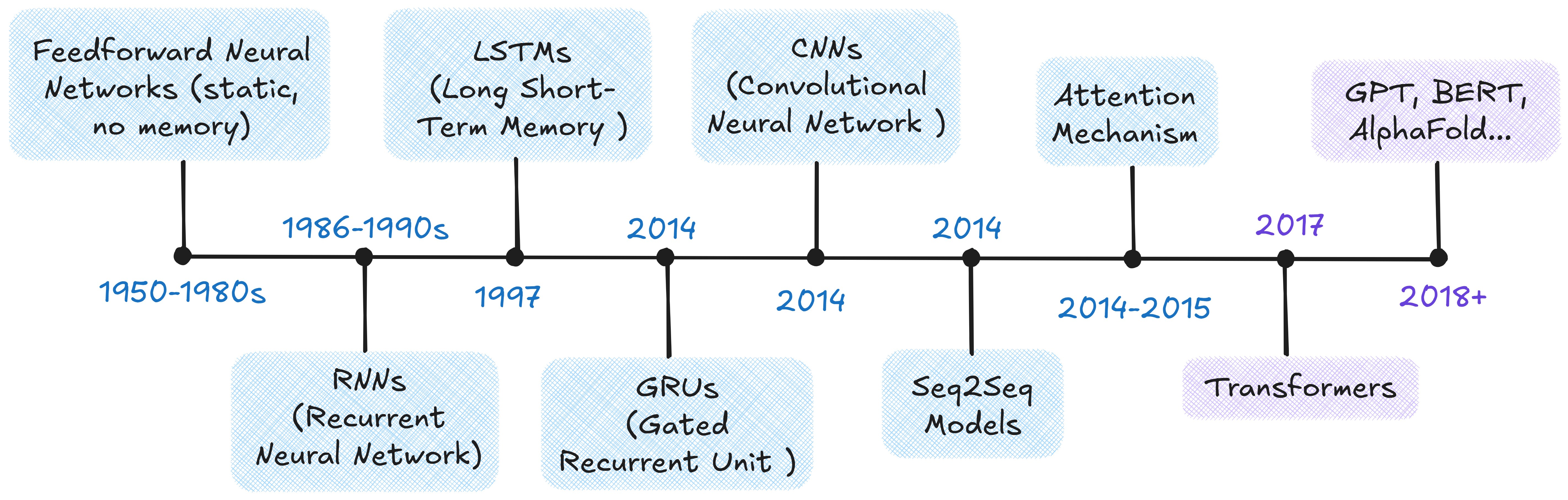
Timeline of Key Language Model Architectures

Evolution of language models: what each introduced and WHY the next was needed
TL;DR — Why Did Transformers Matter?
To summarize the above chart, what were old models missing exactly?
- They struggled with remembering context over long sentences.
- When they tried, they either forgot too quickly or became unstable.
- Models that handled memory better were still slow and hard to scale.
- And compressing whole sequences into one chunk meant losing a lot of detail.
Then came a bold idea: Some Google Brain researchers asked: "What if we removed the whole idea of recurrence from RNNs and CNNs… and just used attention instead?" That simple shift led to the birth of the Transformer — captured perfectly in the title of their paper, "Attention Is All You Need."
What the Transformer changed:
- It let models pay attention to all the words at once (self-attention).
- It trained much faster by processing sequences in parallel.
- It kept word order with positional encodings.
- And it scaled effortlessly — powering GPT, BERT, and today's foundation models.
Transformer Architecture: A Thorough Breakdown
The Transformer is comprised of 2 main building blocks:
- Encoder
- Decoder
Inside these blocks, it relies on 5 core mechanisms that work together:
- Attention (which comes in 4 main variants: self-attention, cross-attention, masked self-attention and multi-head attention)
- Feed-forward networks
- Layer normalization
- Positional encoding (plus the initial input embeddings that convert words into numbers)
- Residual connections
Below is the full original Transformer architecture from the paper Attention Is All You Need (2017). Think of this as a reference point. Don't worry if it looks overwhelming at first. In the rest of this article, I'll break down each component step by step and make sense of how it all fits together.

Transformer Architecture as illustrated in Attention is All You Need (2017). Encoder on the left & Decoder on the right.
We can think of the Transformer as a black box: it takes an input sequence (eg. like a sentence "I like cats" in English) and produces an output sequence (like "J'aime les chats", the same sentence in French). Its power comes from the encoder–decoder structure: the encoder turns the input into a numerical representation, and the decoder uses that to generate the output one token at a time. In the original paper, both the encoder and decoder are shown as stacks of six layers (N=6). Below, I've illustrated this structure, breaking it down into the encoder, the decoder, and their repeating layers.
High-level view of Input -> Transformer -> Output
Slide 1 of 3 - Progressive breakdown of transformer architecture
Attention
Now we've reached the mechanism that's been referenced throughout this article, and the one that powers the core of the Transformer architecture. Introducing...Attention.
Before we talk about attention, here's what you need to keep in mind:
- You now understand how the Transformer turns input sequences into output sequences using encoder and decoder stacks
- Each token in the input becomes a vector (thanks to embeddings), and each layer refines those vectors. (Note: If you aren't familiar with the terms "tokenization" or "word embeddings" then they are explained in an Aside under "Self-Attention" in the article!)
- Unlike older models (as illustrated in the evolution of language models chart), transformers do not rely on memory flowing through time. Instead, they rely on direct connections between all tokens via attention!
Hence, Attention is a mechanism that determines the importance of each component in a sequence relative to every other component in that sequence.
With that being understood, now we'll uncover attention in more detail (which is discussed as 3 different variants in the paper: Self-Attention, Multi-Head Attention, and Cross-Attention.
1) Self-Attention
Say you're given the following sentence: "he swung the bat with incredible force". On its own, the word "bat" could mean either an animal, or a baseball bat. However, the CONTEXT of the sentence is what tells us (and a computer) that it's the baseball bat. Attention helps minimize this ambiguity, by not treating the word (eg. bat) in isolation but by "paying attention" to other words in the sequence.

Attention uses context to resolve ambiguity. Here "bat" means baseball, not the animal.
Before Self-Attention, your input sequence must go through 2 steps: tokenization and token embedding.
Aside on Tokenization & Word Embeddings
1) Tokenization
Computers don't understand words, they understand numbers. So, the first step is to break down a sentence into smaller units called tokens. There are different ways to tokenize text:

Different types of tokenization: breaking text into words, subwords or characters
2) Token Embeddings
Then each of your tokens are mapped to a unique token ID from a pre-defined vocabulary. However, transformers cannot process integers directly; they need vectors. That's where token embeddings come in. An embedding matrix is a giant table:
- V: vocabulary size (the total number of unique tokens a model knows about, eg. 50,000)
- d: embedding dimension (the length of the vector used to represent each token or the number of "features" a token is represented by (eg. 512). It's a hyperparameter of the model.

Turning text into embeddings the model can understand
Each row in this matrix is now a trainable vector representing a token: (example: Transform → Token ID: 1231 → [0.1, 0.3, 0.4, 0.9, 0.8])
Once each input ID is mapped to its embedding, the entire input sentence becomes a 2D tensor!
The key takeaway is that once text is tokenized and mapped into embeddings, each token is now represented as a vector that carries semantic meaning. Similar words or concepts will have embeddings that are close together in this high-dimensional space (eg. bat, swung, hit, ball). These embeddings are what the Transformer operates on.
Attention relies on 3 key inputs for each token (i.e. word in a sequence):
- A Query Vector (Q): what this token wants to find out
- A Key Vector (K): what this token offers to others
- A Value Vector (V): the actual content this token can contribute to
Here's an analogy to intuitively understand Q, K and V vectors:
- Picture doing a simple Google Search. The Query is what you type into the search bar (i.e. "how do transformers work?"), the Key are the titles of webpages stored by the data engine, and the Value are the actual content of those.
In self attention, the Query, Key and Value matrices are all derived from the same input vector. They are calculated by a matrix multiplication of the input vector (X) and a learnt weight matrix (W) for each Q, K and V matrix. The weight matrix (W) is learnt on the loss function of the transformer during backpropagation.

How Query, Key and Value matrices are derived
After you type something into Google, you want the search engine to match your query against page titles and keywords to find the most relevant results. In a transformer, this is exactly what happens when your query vector is compared against the key vectors...the model needs a way to measure which ones are most similar or relevant. This is done using a compatibility function, which is nothing other than the "dot-product" (a simple yet powerful way to check how aligned 2 of your vectors are). The results of these comparisons are laid out in a compatibility matrix, where higher dot product values indicate a stronger match between a query and a key.

Compatibility matrix showing how aligned query and key vectors are. Every cell marked "high" is likely to score high in compatibility (i.e. higher dot-product value)
When working with very high-dimensional vectors, the dot products between queries and keys can become extremely large. This creates a problem during backpropagation: those large values cause the gradients to shrink down to very small numbers, a well-known issue called the vanishing gradient problem. To prevent this, the dot products are scaled down by dividing them with the square root of the key dimension (√dₖ). This adjustment keeps the values at a manageable range and stabilizes training.
Once the dot products are scaled, the next step is to turn them into meaningful weights that reflect how much attention each token should get. To do this, the transformer applies a softmax function to the scaled values. Softmax normalizes the numbers so that they all fall between 0 and 1, and ensures that the weights for each query sum up to 1. In other words, it transforms raw scores into a probability distribution across tokens. The result is what we call the attention weight matrix, shown below:

Softmax normalizes compatibility scores so they can be interpreted as attention weights.

A hypothetical self-attention heatmap and score matrix for the sentence "He swung the bat with incredible force." The numerical scores (matrix) are visualized as color intensities (heatmap). The weights are fabricated to illustrate how tokens might attend to one another in a Transformer layer. Note: darker cells indicate stronger attention.
The last step of the self-attention mechanism is multiplying the attention scores by the value matrix. This matrix carries the word embeddings for each token in the input sequence, holding the actual information each word contributes. Once the value matrix is multiplied by the softmax of the attention scores, the output becomes a new representation that captures both the meaning of each word and its context within the sequence.

Formula for self-attention in transformers
And that's self-attention explained in a nutshell!
2) Multi-Head Attention
So far, self-attention lets a model figure out which words in a sentence matter most to each other. But what if there's more than one kind of relationship worth noticing at once? For example, in "He swung the bat with incredible force," one relationship connects "swung" ↔ "bat" (the action and object), while another connects "incredible" ↔ "force" (description and intensity). Multi-headed attention lets the model look at all those relationships in parallel. Each head learns a slightly different way of paying attention. One might focus on grammar, another on meaning, another on emotion...and when you combine them, you get a much richer understanding of the sentence.
From a computational perspective, this happens by running multiple attention heads simultaneously (eight in the original Transformer paper), then concatenating their results and passing them through a final projection matrix, W0. This projection blends the insights from every head into a single, context-aware representation.

Each attention head computes its own set of Q, K, and V projections, produces an attention output, and all heads are then concatenated and projected through W0 to form the final output
Why 8 Attention Heads?
Eight isn't a fixed rule, it's a hyperparameter that balances expressiveness and efficiency. If the model's embedding size is 512 and you use 8 heads, each head gets 64 (512 ÷ 8) dimensions for its queries, keys, and values. That means every head operates on a lower-dimensional view of the input, and together they cover multiple subspaces that the model later recombines.
- Too few heads → each one must learn too many relationships at once, reducing specialization.
- Too many heads → each becomes too small to represent anything meaningful (and inference gets slower and more compute-heavy).
In practice, 8 heads hits a good spot: diverse enough to learn multiple contextual patterns, yet large enough per head to retain useful capacity.
Now that we understand how attention operates in a single layer, let's explore how it's used differently inside the encoder and the decoder. The encoder uses self-attention, while the decoder uses 2 stacked forms: masked self-attention and cross attention. I'll be explaining these 2 nuanced decoder attention mechanisms below:
3) Masked Self-Attention (Decoder-Side)
In the decoder, the first attention layer is slightly modified, it's called: masked self-attention.
In regular self-attention, every token can "see" every other token in the sequence, which works perfectly for the encoder (since the entire input is known).
Here, the same self-attention mechanism applies, but with a twist: the model is forbidden from looking at future tokens when predicting the next word.
To enforce this, a look-ahead mask is applied to the scaled dot-product score matrix, setting all entries above the diagonal to negative infinity before softmax. This ensures that each token can only attend to previous ones, preserving the autoregressive property of language generation, so the model writes strictly left-to-right (just like we do).
Note: Why do we use negative infinity when masking? Because softmax turns those values into 0! (You're basically telling the softmax function that these positions don't exist)

Applying the look-ahead mask during masked self-attention. Future positions are set to −∞ before softmax, ensuring each token only attends to itself and prior tokens.
💭 What happens if we didn't have masking?
- The model would already see the correct future tokens when predicting the next word, so instead of learning to anticipate what comes next, it would simply copy information it shouldn't know yet.
- It would achieve a perfect training loss — since every prediction would be trivially correct — but it would never actually learn how to generate text step-by-step.
- During inference, it would completely collapse: without the ability to "think ahead" on its own, it wouldn't know what to predict next.
4) Cross Attention (Decoder-Side)
After the decoder finishes attending to its own generated tokens through masked self-attention, it still needs a way to connect back to the input sentence the encoder processed. That's where cross-attention comes in. It acts as a bridge between the encoder and decoder, letting the decoder "look over" at the encoder's output to decide which parts of the input matter most for generating the next word.
There are actually two sequences involved:
- Source sentence → processed by the encoder
- Target sentence → generated by the decoder
During training, the input to the decoder is the target sequence shifted one position to the right, starting with a special beginning-of-sentence token (<start>).
This ensures each output position only receives previous tokens, not the token at the same position.
That behavior is enforced by the shift + self-attention mask working together.
Mechanically:
- The encoder's output provides the key (K) and value (V) to the decoder's second multi-head attention layer.
- The query (Q) comes from the decoder's own hidden states (based on what's been generated so far).
So instead of attending within the same sequence like in self-attention, the decoder is now attending across sequences, aligning what it's generating with what the encoder understood.

During training, the encoder receives the source sentence, and the decoder receives the target sentence shifted one position to the right. This shift, along with masking, ensures the decoder predicts each word based only on previously seen tokens.
Feed-Forward Neural Networks
Once attention has done its job capturing relationships between tokens and layering in contextual meaning, the Transformer passes that information through a Feed-Forward Neural Network (FFN).
You can think of the FFN as the processing unit of each layer. While attention tells the model what to focus on, the FFN decides what to do with that information. Every token in the sequence is passed through the same small neural network independently, applying non-linear transformations that help the model detect deeper and more abstract features.
Architecture
The FFN in each encoder and decoder layer consists of two linear transformations with a non-linear activation function applied between them.

Mathematical form of the Feed-Forward Neural Network in each Transformer layer

Inside the Transformer's Feed-Forward Layer
1) Expansion: The first linear layer projects the input vector x from the model's embedding dimension (d_model) to a larger intermediate dimension (dff).
In the original Transformer paper, dff was set to 4 times the dimension as d_model (eg. 512 → 2048). This expansion allows the model to learn more complex features.
2) Non-linear Activation: An activation function is applied to the output of the first transformation. This step introduces non-linearity, which gives the model expressive power. Without it, stacking multiple Transformer layers would still behave like one big linear transformation, and limit the model's ability to capture complex relationships. Earlier transformer models used ReLU.
3) Contraction: The second linear transformation then "contracts" the expanded representation back to the original model dimension (d_ff → d_model). This ensures that the output has the same dimensionality as the input.

Feed-Forward Network (FFN): Expands each token's vector (512 → 2048) through a linear layer, applies a non-linear activation (e.g. ReLU), and compresses it back (2048 → 512).
Layer Normalization
Training deep models like Transformers is hard. They contain billions of parameters, and gradients can easily explode or vanish as signals move through layers. To stabilize learning, Transformers use Layer Normalization.
Normalization helps by scaling activations so that their mean is 0 and standard deviation is 1. This keeps every layer's outputs within a steady range, preventing some neurons from dominating while others fade out. In simple terms, it ensures that learning happens smoothly and consistently across ALL features.
Unlike Batch Normalization, which normalizes across a batch of examples, Layer Normalization works within each data point, where it normalizes across the features of a single token. That's why it's ideal for Transformers, where batch sizes or sequence lengths can vary!

Layer Normalization rescales each token's activations so that their mean is 0 and variance is 1. This keeps learning stable by preventing gradients from exploding or vanishing, while the learnable parameters (γ and β) let the model fine-tune how much to scale or shift the result
Residual Connections
We've now covered the following mechanisms: Attention for context, the FFN for deep feature transformation, and Layer Normalization for stability.
But think back to when we discussed the problem of vanishing gradients (the reason we scale the dot products in Attention). While Layer Normalization helps stabilize things, it doesn't fully solve the issue of building truly deep, stable models.
How do you make a model that's over ten to hundreds of layers deep, without the early layers forgetting how to learn? The answer is residual connections!
Imagine a pipeline where water has to flow through ten layers of filter paper. By the time it reaches the last layer, the pressure is incredibly low. Similarly, in a deep neural network, information (and the learning signal, the gradient) can degrade and fade as it passes through sequential layers. This can lead to 2 problems:
- 1) Vanishing Gradients: The learning signal dies before reaching the layers closest to the input.
- 2) Identity Crisis: Each layer is forced to learn the entire complex function from scratch, which is incredibly difficult for the optimization algorithm
The solution is to create a direct bypass known as residual or "skip" connections around every sublayer (in a transformer, this is applied around both the Multi-head attention block and the Feed Forward Neural-Network block.

The Core Residual Mechanism: Add & Norm. The x bypasses the sub-layer F(x) and is added to its output, followed by Layer Normalization (LayerNorm). This crucial step stabilizes learning in deep Transformer stacks
This residual connection is is the line you see above running around the main block. It is a direct path that lets information and gradients flow smoothly through the network. This simple addition (x and sublayer F(x)) prevents information loss, keeps gradients stable during training, and helps the model converge faster! Without residual connections, Transformers simply wouldn't be trainable.
Positional Encoding
So far, we've covered what the Transformer pays attention to, but not where.
Unlike RNNs, which process tokens sequentially, Transformers see the entire input at once. That parallelism is what makes them so fast...but it also means they lose any built-in sense of order.
To fix this, we inject positional encodings: extra signals that tell the model where each token is in the sequence. Each token's embedding is combined with a positional vector of the same dimension, giving the model two pieces of information:
- 1. What the token represents (its meaning), and
- 2. Where it appears (its position).

Each input embedding is combined with a positional encoding to represent both meaning and sequence
Each token position produces a wave-like pattern across embedding dimensions. Together, these overlapping sine and cosine functions form a unique "positional fingerprint" for every token.
Each embedding dimension oscillates at a different frequency. Low-frequency waves capture broad, global structure (like "beginning vs end"), while high-frequency waves capture finer details ("next token vs previous one").
When added to token embeddings, these waves create unique signatures for each position. Since sine and cosine are continuous, the model can infer relative distances between tokens. This lets the Transformer generalize to sequences longer than any it saw during training.
To make this concrete, here's a smaller example with d = 4 showing how each token ("Transformers are cool") gets its own positional encoding vector:

Positional encoding with d=4: each position is represented by interleaved sine and cosine values at varying frequencies, allowing the model to infer relative and absolute position.
And...that's it. That completes the full transformer architecture!
Final Remarks!
If you've made it this far, I hope you can now see how the Transformer came to life! From the long history of models that led up to it, and why every design choice exists the way it does. Every part of it: attention, feed-forward networks, layer normalization, came from fixing something the last generation couldn't.
Now that you understand the foundation, you can actually dive into the fun stuff. You'll be able to read about attention optimization techniques like FlashAttention, Sparse Attention, or Grouped Query Attention and know what they're improving. You'll understand how the FFN evolves into Mixture-of-Experts (MoE), and how newer models use Rotary Positional Embeddings (RoPE) instead of fixed sinusoids & why that works.
All of this makes way more sense once you've built a solid mental picture of the original Transformer. That's what this piece was meant to do. It took me months to research, refine, and hand-illustrate, and I hope it gave you the kind of clear, visual understanding I once wished I had.
The Transformer isn't just a model. It's a story of small, clever ideas stacked over time - each one bringing us closer to teaching machines how to understand us. You now understand the foundation that powers almost every modern AI model. From here, the frontier's yours to explore :)))
© All diagrams and illustrations in this article were hand-drawn and belong to Krupa Dave.
References
- Vaswani et al., "Attention Is All You Need." arXiv:1706.03762
- Bahdanau et al., "Neural Machine Translation by Jointly Learning to Align and Translate." arXiv:1409.0473
- He et al., "Deep Residual Learning for Image Recognition." arXiv:1512.03385
- Jay Alammar, "The Illustrated Transformer." jalammar.github.io
- Alejandro Ito Aramendia, "Attention Is All You Need: A Complete Guide to Transformers." Medium
- StatQuest with Josh Starmer, "Transformers Explained Visually." YouTube
- Roy Swastik, "Transformer Tokenization and Vocabulary Creation." Hugging Face Blog
- Stack Overflow, "Transformer 'Attention Is All You Need' Encoder-Decoder Cross-Attention Explanation." Stack Overflow Thread
- AI Research Studies, "History of Large Language Models: From 1940 to 2023." ai-researchstudies.com
- DataCamp, "Feed-Forward Neural Networks Explained." datacamp.com