Extending That XOR Trick to Billions of Rows

Jul 3, 2025

Can we extend the XOR trick for finding one or two missing numbers in a list to finding thousands of missing IDs in a billion-row table?

Yes, we can! This is possible using a data structure called an Invertible Bloom Filter (IBF) that compares two sets with space complexity based only on the size of the difference. Using a generalization of the XOR trick [1], all the values that are identical cancel out, so the size of this data structure depends only on the size of the difference.

Most explanations of Invertible Bloom Filters start with standard Bloom filters, which support two operations: insert and maybeContains. Next, they extend to counting Bloom filters, which enables a delete operation. Finally, they introduce Invertible Bloom Filters, which add an exact get operation and a probabilistic listing operation. In this article, I will take a different approach and build up to an IBF from the XOR trick.

IBFs have remained relatively obscure in the software development community while the XOR trick is a well-known technique thanks to leetcode. My goal with this article is to connect IBFs to the XOR trick so that more developers understand this fascinating and powerful data structure.

Finding 3 Missing Numbers

Let's start with a concrete example:

A = [1,2,3,4,5,6,7,8,9,10] B = [1,2,4,5,7,8,10]

Set B is missing 3 numbers: {3, 6, 9}.

The classic XOR trick works for finding 1 or 2 missing numbers, but what about 3 or more? If we don't know how many numbers are missing, we can use a count field to detect when the usual XOR trick will fail:

XOR(A) = 1 ^ 2 ^ ... ^ 10 = 11 COUNT(A) = 10 COUNT(B) = 7

Since B has 7 elements and A has 10, we know 3 numbers are missing—too many for the basic XOR trick.

To work around this limitation, we can partition our sets using a hash function. Let's try with 3 partitions:

H(1) = 2, H(2) = 1, H(3) = 1, H(4) = 0, H(5) = 0 H(6) = 0, H(7) = 2, H(8) = 1, H(9) = 2, H(10) = 1 A_0 = [4,5,6] B_0 = [4,5] A_1 = [2,3,8,10] B_1 = [2,8,10] A_2 = [1,7,9] B_2 = [1,7]

Now each partition has at most 1 missing element, so we can apply the XOR trick to each:

XOR(B_0) ^ XOR(A_0) = (4 ^ 5) ^ (4 ^ 5 ^ 6) = 6 XOR(B_1) ^ XOR(A_1) = (2 ^ 8 ^ 10) ^ (2 ^ 3 ^ 8 ^ 10) = 3 XOR(B_2) ^ XOR(A_2) = (1 ^ 7) ^ (1 ^ 7 ^ 9) = 9

Success! We recovered all 3 missing elements: {3, 6, 9}.

Unfortunately, this approach alone doesn't work in practice. Here, we got lucky with our hash function. Usually, elements will not distribute evenly across partitions, and some partitions might still have multiple differences.

Detecting when the XOR trick fails

To fix the problems with naive partitioning, we will need to use a more sophisticated approach.

Let's generalize beyond "missing numbers" to the concept of symmetric difference. The symmetric difference of two sets A and B is the set of elements that are in either set but not in both: (A \ B) ∪ (B \ A), often written as A Δ B.

Figure 1: The symmetric difference A Δ B includes elements that are in either set A or set B, but not in both sets.

Consider this example:

A = [1,2,3,4,6] B = [1,2,4,5]

The symmetric difference is {3, 6, 5}—elements 3 and 6 are only in A, while element 5 is only in B.

The naive approach of checking |COUNT(A) - COUNT(B)| = 1 fails here because the count difference is 1, but the symmetric difference has 3 elements. Applying the basic XOR trick gives a meaningless result.

To detect this case, we can use an additional accumulator with a hash function:

COUNT(A) = 5, XOR(A) = 2 COUNT(B) = 4, XOR(B) = 2 XOR_HASH(A) = H(1) ^ H(2) ^ H(3) ^ H(4) ^ H(6) XOR_HASH(B) = H(1) ^ H(2) ^ H(4) ^ H(5) XOR(B) ^ XOR(A) = 0 XOR_HASH(B) ^ XOR_HASH(A) = H(3) ^ H(5) ^ H(6) H(3) ^ H(5) ^ H(6) ≠ H(0)

While we can't yet recover the full symmetric difference, we can detect when the XOR result is unreliable by checking if the hash accumulators behave consistently.

Invertible Bloom Filters

The Core Idea

The original XOR trick relies on an accumulator that stores the XOR aggregate of a list. Building on this, we've introduced:

1. Partitioning to divide sets into smaller parts
2. Additional accumulators that store the element count and hash of XOR aggregate

To fully generalize this into a robust data structure, we need:

1. A partitioning scheme that creates recoverable partitions with high probability
2. An iterative process that uses recovered values to unlock additional partitions

This is exactly what Invertible Bloom Filters [2] provide. IBFs use a Bloom filter-style hashing scheme to assign elements to multiple partitions, then employ a graph algorithm called "peeling" to iteratively recover the symmetric difference with very high probability [3].

Structure

An IBF consists of an array of cells, where each cell contains three accumulators:

• idSum: XOR aggregate of element values
• hashSum: XOR aggregate of element hashes
• count: number of elements in the cell

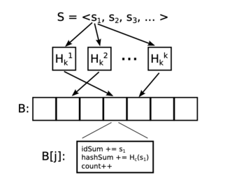Figure 2: Figure from [2] showing the process of encoding elements into IBF cells.

Operations

For computing symmetric differences, IBFs support three key operations:

1. Encode: Build an IBF from a set of values
2. Subtract: Subtract one IBF from another—identical values cancel out, leaving only the symmetric difference
3. Decode: Recover stored values by finding "pure" cells (count = ±1 and H(idSum) = hashSum) and iteratively "peeling" them

The IBF has one parameter d—the expected size of the symmetric difference. With proper sizing (typically m > 1.22d cells), IBFs recover the full symmetric difference with very high probability.

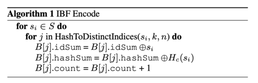
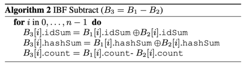
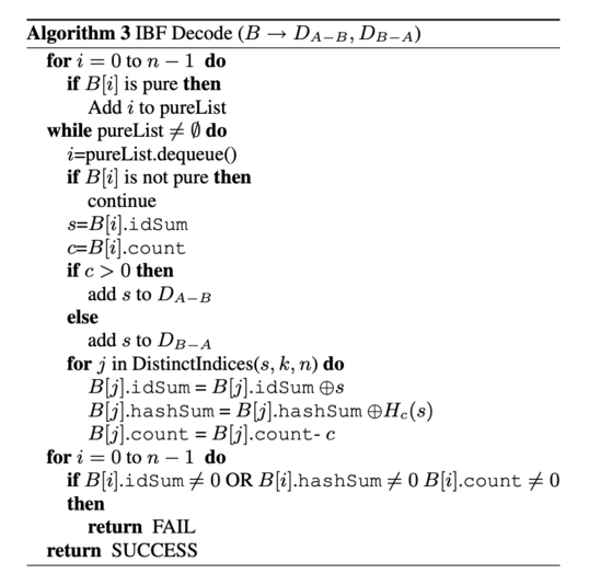Algorithms for each IBF operation from [2].

Example Implementation

I have not found a solid, maintained library of IBFs in any language (if you know of any please let me know!), so I created a basic implementation in Python if you would like to play with it: https://gist.github.com/hundredwatt/a1e69ff300de941041d824e49249d3d7

Example usage:

a = [1, 2, 4, 5, 6, 7, 9, 10] b = [1, 3, 4, 5, 6, 7, 9, 10] set_a = set(a) set_b = set(b) ibf_size = 100 k = 4 ibf_a = IBF(size=ibf_size, k=k) for item in a: ibf_a.insert(item) ibf_b = IBF(size=ibf_size, k=k) for item in b: ibf_b.insert(item) diff_ibf = ibf_a.subtract_ibf(ibf_b) success, decoded_added, decoded_removed = diff_ibf.decode() assert(success) expected_added = set_a - set_b expected_removed = set_b - set_a print("--- Verification ---") print(f"Expected added (in A, not B): {len(expected_added)} items") print(f"Decoded added: {len(decoded_added)} items") assert(expected_added == decoded_added) print(f"Expected removed (in B, not A): {len(expected_removed)} items") print(f"Decoded removed: {len(decoded_removed)} items") assert(expected_removed == decoded_removed)

About the "Set Reconciliation" Problem

The general problem of efficiently comparing two sets without transferring their entire contents is called "set reconciliation." Early research used polynomial approaches [4], while modern solutions typically employ either Invertible Bloom Filters or error-correction codes [5].

Conclusion

IBFs are a powerful tool for comparing sets with space complexity based only on the size of the difference. I hope this article has helped you understand how IBFs work and how they can be used to solve real-world problems.

If you want to learn more about IBFs, I recommend reading the references below. The "Further Reading" section contains some additional, advanced papers that I found interesting.

If you have any questions or feedback, please feel free to reach out to me, contact info is in the footer.

References

[1] Florian Hartmann, "That XOR Trick" (2020), https://florian.github.io/xor-trick/

[2] David Eppstein, Michael T. Goodrich, Frank Uyeda, and George Varghese, "What's the Difference? Efficient Set Reconciliation without Prior Context," SIGCOMM (2011), https://ics.uci.edu/~eppstein/pubs/EppGooUye-SIGCOMM-11.pdf

[3] Michael Molloy, "Cores in Random Hypergraphs and Boolean Formulas," Random Structures & Algorithms (2003), https://utoronto.scholaris.ca/server/api/core/bitstreams/371257de-0a44-4702-afeb-542ae9a06986/content

[4] Yaron Minsky and Ari Trachtenberg, "Set Reconciliation with Nearly Optimal Communication Complexity" (2000), https://ecommons.cornell.edu/server/api/core/bitstreams/c3fff828-cfb8-416a-a28b-8afa59dd2d73/content

[5] Pengyu Gong, Lei Yang, and Liwei Wang, "Space- and Computationally-Efficient Set Reconciliation via Parity Bitmap Sketch," VLDB (2021), https://vldb.org/pvldb/vol14/p458-gong.pdf

Further Reading

• Invertible Bloom Lookup Tables, Mitzenmacher (2011), https://people.cs.georgetown.edu/~clay/classes/fall2017/835/papers/IBLT.pdf

This paper extends the original IBF paper to support additional encoded fields (not just a single idSum) and a more robust decoding algorithm that I found to be necessary for production use.

• Simple Multi-Party Set Reconciliation, Mitzenmacher (2013), https://arxiv.org/abs/1311.2037

This paper shows how to extend IBF-based reconciliation to efficiently handle three or more parties. The implementation is neat, it encodes the IBFs on finite fields of a dimension equal to the number of parties.

• Simple Set Sketching, Bæk (2022), https://arxiv.org/abs/2211.03683

This paper reduces the size of the IBF by eliminating the hashSum field. Instead, it uses a hash function that calculates the cell index as a checksum and has some additional checks in the decoding process to deal with potential "anomalies" that show up in this approach.

• Practical Rateless Set Reconciliation, Yang (2024), https://dspace.mit.edu/handle/1721.1/156671

Standard IBFs require knowing the expected size of the symmetric difference beforehand to size the filter correctly. This recent work introduces "rateless" IBFs that adapt their size dynamically, making them more practical when the difference size is unknown or highly variable.