Field Guide to TSL and WebGPU

Now supported in Apple's most recent version of iOS and Safari ¹, WebGPU is finally gaining widespread support, allowing for more advanced 3D capabilities on the web. As someone working with WebGL on the side, this was the push I needed to, at last, dedicate some time to learning more about this new set of APIs and see how I could port over some of my existing WebGL/shader knowledge and work to it.

This work involved not only familiarizing myself with WGSL, the shader language designed for WebGPU, but also TSL: Three.js's higher-level, JavaScript-like shading language. Moreover, WebGPU also introduces some new constructs, such as compute shaders, a new, exciting, yet nebulous type of shaders that seemed like it could improve some key aspects of my workflow.

To guide me through this learning journey, I decided the most practical way would be to spend my summer porting over key projects I've worked on throughout the years, such as my glass material, post-processing, particles, as well as several other fun shader experiments. There were numerous gotchas and undocumented features, which sometimes made the experience quite frustrating, but in the end, I managed to familiarize myself with these new tools and build beautiful scenes with them.

This article is a compilation of the steps I took, going from knowing very little about TSL and WebGPU to becoming comfortable with them, and, as a result, serves as the field guide I wish I had. In it, I will tell you all about these new tools/APIs and the role they play while also sharing recipes to implement some essential components of a 3D scene, whether it is to build a simple material using TSL's new node system, or to leverage compute shaders in diverse use cases like instanced meshes, particles, or post-processing effects.

If, like me, you've seen the names TSL or WebGPU used interchangeably, you may be confused about their roles and how they relate to one another. This first part should answer all your questions regarding these two concepts so you can start building on your own with solid foundations.

TSL and WebGPU

Many creative developers were very excited about the recent expansion of WebGPU support, and for good reason: this new API set brings the web up to par with modern graphics API like Vulkan or Metal, the backbone of many professional creative software and game engines. It provides lower-level controls (memory allocation, bind groups, etc.) and offers new constructs such as compute shaders, while having near native performance ².

On the other hand, my fellow Three.js developers were also getting interested in something a bit different, yet loosely related: the Three.js Shading Language. A functional language based on JavaScript that is meant to act as a sort of umbrella shading language, making shader creation more accessible and also maintainable over time. Through the introduction of TSL, Three.js provided the ability to write shaders that can run on WebGPU, which was not supported up to that point, while also allowing for these same shaders to run on WebGL, thus letting developers target any platform with unique code, regardless of WebGPU support ³

Below is an example of a simple shader written in TSL and its GLSL and WGSL equivalents:

As you can see, the syntax is very (not to say "extremely") functional, even for simple operators. While this offers the ability to target WebGL or WebGPU alike, to me, it comes with the sacrifice of legibility. I guess it's a matter of taste and habit. If this bothers you a bit too much, you can still opt for the glslFn and wgslFn TSL function to write native code, however, you still have to rely on TSL at the end of the day to define and consume those shader chunks in your materials/effects through its Node System.

Thus, to summarize:

• You can use TSL to write shaders for both WebGL and WebGPU.

• You still can use GLSL and RawShaderMaterial/ShaderMaterial if you want, but you'll always be limited to WebGL.

• You cannot write raw WebGPU shaders the same way you can in WebGL: it's all abstracted away by TSL.

The Node System

While the abstraction layer and the lack of ability to write raw WebGPU shaders were a bit of a bummer to me as I tend to prefer using low-level constructs, TSL's Node System is, to me, a key feature that sold me on it and made me embrace it.

Until now, when we wanted to modify an existing material in WebGL, even for the smallest of changes, we had to painstakingly work our way through string concatenation of several shader chunks using the onBeforeCompile method.

Today, TSL provides hooks for each of its NodeMaterials, such as colorNode, normalNode, or positionNode, to respectively modify the color, normals, and vertex position output of your material very easily. Even better, every stock Three.js material now has a "node equivalent" compatible with this new API:

• MeshStandardMaterial has MeshStandardNodeMaterial

• MeshBasicMaterial has MeshBasicNodeMaterial

• MeshPhysicalMaterial has MeshPhysicalNodeMaterial

and so on.

Diagram illustrating an arbitrary set of nodes for a given material and a representation of the data they can override.

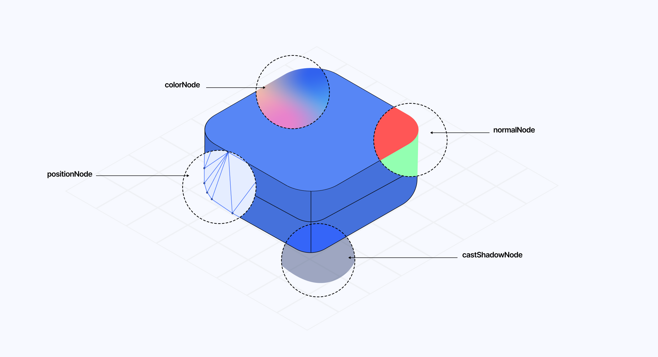
Of course, there are other nodes I did not list here, and many more to come as TSL expands its feature set. The ones mentioned are, to me, the most important and the first you will encounter when playing with TSL and shaders.

As we ease into our WebGPU and TSL journey, let’s start by setting up our WebGPURenderer with React Three Fiber and recreating some classic shader examples you might have come across online, or that I walked through in past blog posts.

Using the WebGPU renderer

To get access to the new WebGPU features, we first need to instantiate its renderer in our React Three Fiber project through the gl prop of the Canvas component. Luckily, Canvas has been updated in React Three Fiber v9 to support an asynchronous gl prop ⁴, a necessary feature since the WebGPURenderer requires async initialization.

The following code snippet showcases how we will initialize React Three Fiber projects featuring WebGPU features going forward:

While initializing WebGPURenderer may give the impression that we made an arbitrary decision to make our 3D scene WebGPU-only, that is, in fact, not the case. WebGPURenderer supports both WebGPU and WebGL, and will fall back to WebGL when WebGPU is not available on the device attempting to render the scene.

If, throughout the development of your scene, you want to ensure that it still functions correctly in WebGL, you can pass the forceWebGL: true parameter to your WebGPURenderer.

The demo below sets up a React Three Fiber scene powered by WebGPU, including some simple shaders written with TSL. You can try forcing it to render with WebGL and see for yourself that it will yield the same result, which is one of the key advantages of writing shaders with TSL.

Displacement and Normals

As a first, more elaborate example, we will create a classic blob by introducing some organic and dynamic displacement to the sphere at the center of the previous scene. To make it ambitious and highlight the benefits of TSL and its node system, we can try to do all of this on top of meshPhongNodeMaterial by writing a shader for:

• the positionNode, to modify the position of vertices over time

• the normalNode, to adjust the normal data of our sphere accordingly so the lighting and shadows of our moving sphere match the displacement of its vertices

all of that while maintaining some of the key physical properties that are core to this material.

To organize my TSL code, I like to:

• Wrap them all up inside a useMemo.

• Export a nodes property that will contain a field for each of our TSL shaders.

• Export a uniforms property that will contain all the uniforms we want to adjust.

This provides a more structured approach to organizing our TSL code within our React code, ensuring that key constructs such as uniforms are not accidentally recreated.

We will start by writing a custom positionNode to modify the position of the vertices of our sphere mesh following a noise. I transpiled an implementation of Perlin Noise using the transpiler that we'll use in this example, it will be fully featured in the playground at the end of the section.

To animate our blob over time, we would want to pass a time uniform to adjust the positions of the vertices over time. However, between WebGL and WebGPU, uniforms work a bit differently:

• WebGL uniforms are global variables that you can set directly by calling gl.uniforms and call it a day.

• WebGPU uniforms live in a uniform buffer, which requires explicit memory allocations ⁵.

This difference between convenience and control is hidden from us by TSL: to declare your uniforms, use the uniform function. And that, regardless of whether we write our position shader using the TSL syntax or GLSL/WGLSL syntax.

Now we can work our way towards recomputing normals. We did something similar in Shining a light on Caustics with Shaders and React Three Fiber, where we had to resort to modifying the shader code of the source material quite heavily and had to be very rigorous about it to ensure we would not break some of its key features. Thanks to the node system, we now simply need to:

• Expand the positionNode to compute the displaced normals.

• Send the recomputed normals through a varying

• Declare a normalNode where we can return that data to be consumed by the material

Like uniforms, varying behavior also differs between WebGL and WebGPU, and thus, once again, we need to rely on a TSL function to hide the complexity from us.

Now that we declared all the nodes we need alongside their respective shaders, all we need to do for our mesh to leverage them is to pass each node to its corresponding node prop in our node material:

As you can see, the days when we needed to use onBeforeCompile and a series of complex string concatenation to modify the shader code within Three.js' materials are long gone. We can now rely on the node system to make those modifications on top of existing materials without too much mess. The demo below showcases the result of the code we established above:

Glass Material

In this section, let's increase the complexity level up a notch and not only see what it takes to build a material from scratch, but also:

1. How to handle textures as a uniform.

2. The subtle differences and gotchas between writing the material in TSL vs WGSL

Indeed, something I omitted to tell you in the previous part is that the uniform function only supports the following types: boolean | number | Color | Vector2 | Vector3 | Vector4 | Matrix3 | Matrix4, type = null. This may be a bit confusing at first, especially after building WebGL shaders and routinely passing textures as uniforms for all our experiments. Instead, we will need to leverage the texture TSL function.

I'm not going to lie, I was a bit puzzled here with this texture function and still am a bit as of writing those words due to its usage:

• On the one hand, you can use it to retrieve a texel at a specific UV in your TSL code.

• On the other hand, I also found myself using it as a way to pass a texture as a uniform to a shader written in WGSL, as it was the only way to convert my THREE.Texture type to a proper ShaderNodeObject<THREE.TextureNode> type, which my shader required for texture sampling (technically a texture_2d<f32>).

The following code snippets illustrate this dichotomy, which has lost me quite a few times already:

I'm talking a lot about textures in this part because they are the backbone of my custom implementation of a glass material, which I've documented in Refraction, Dispersion, and other shader light effects. Below is a code snippet featuring its implementation in TSL, on which I want to highlight the following:

• The ability to split your TSL into as many functions as you wish by simply declaring them with the Fn function. You can pass arguments to them as objects if you want to have specific names for your variables, or as elements in an array if you prefer them inline.

• The ability for your shader to reference global constants from your JavaScript/React code, without necessarily having to send it as a uniform (e.g. like lightPosition).

The WGSL equivalent is a bit different but interesting nonetheless:

• You can use the code TSL function to split your WGSL shaders into reusable bits; however, the main entrypoints need to use wgslFn.

• Your texture_2d<f32> from your WGSL function becomes a ShaderNodeObject<THREE.TextureNode>, so you need to first call texture with the texture you want to sample as an argument.

• Shaders written using the wgslFn or glslFn TSL function seem to always require to have their set of arguments passed as an object.

The demo below showcases the glass material built in TSL and working on top of the blob that we implemented in the first part.

Now that we have a better grasp of TSL and know how to leverage it to use and write shaders for the new WebGPURenderer, we can bring our focus to one of the headline features of WebGPU that many developers were excited about: compute shaders.

There are now two pipelines we can leverage to build our 3D scenes:

• The render pipeline, used for drawing graphics, is the same as the one we're familiar with in WebGL.

• The compute pipeline, designed for more general-purpose computation that can be run on the GPU ⁶.

The latter consists of a single compute shader stage (no vertices, no rasterization, no fragments) in which:

1. We take in arbitrary input data such as textures or buffers.

2. Execute workgroups of threads, or shader invocations, to process those inputs a function defined as a compute shader.

3. Output the resulting data in one or multiple buffers. We can feed those resulting buffers to the render pipeline or back to the CPU.

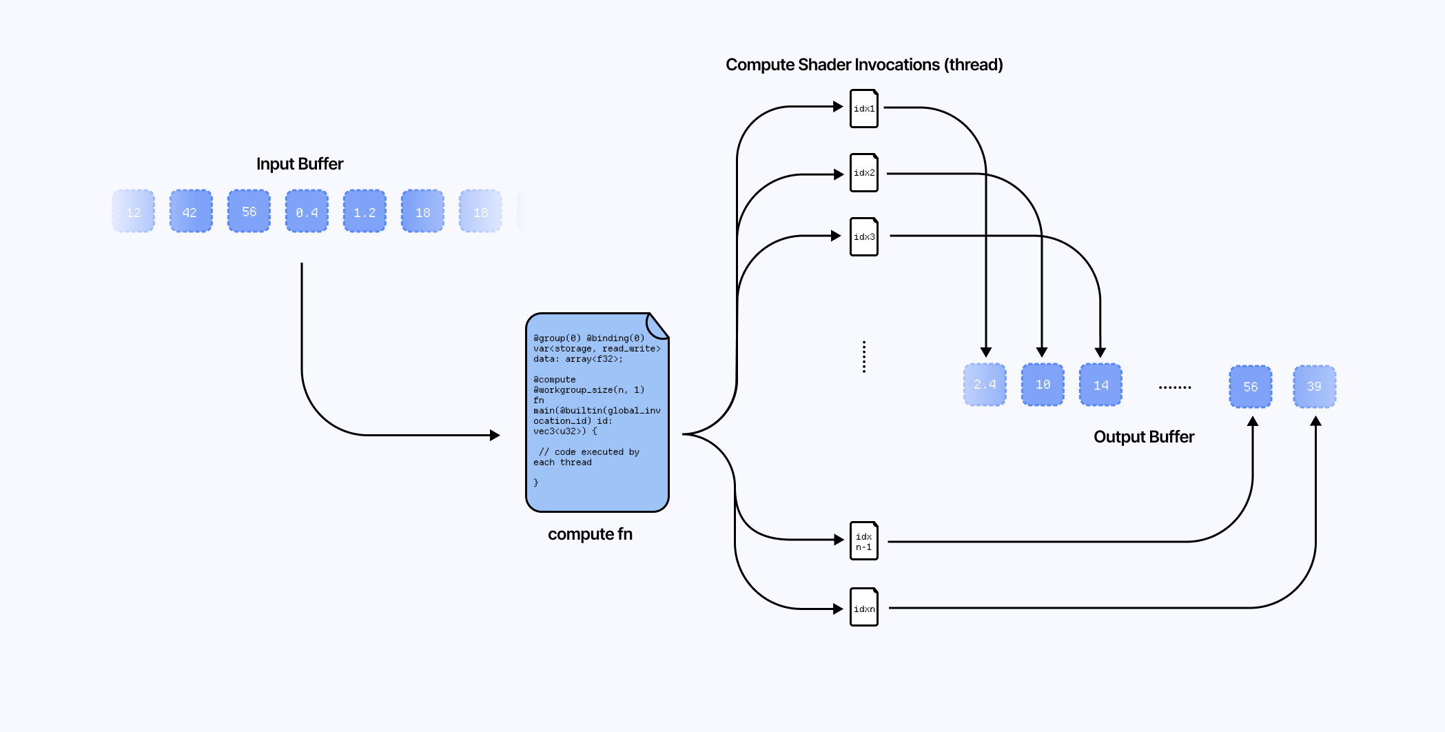
While our render pipeline shaders are tied to draw calls and rasterization, we can call/execute our compute shaders programmatically, thus letting us decide when and how many times they run.

Creating Compute Shaders in TSL

Let's examine a first example of how to leverage the compute pipeline in TSL. We'll do a matrix multiplication on the GPU using compute shaders and read back its result on the CPU. Like our previous shader code, we can declare our compute shader either directly in TSL or with the wgslFn function:

We then need to call our compute shader TSL function by dispatching it using the .compute method.

The resulting computeNode can then be invoked at any time with the gl.computeAsync or gl.compute methods. In the following example, we call it at render time, where we also retrieve the result of our operation using the gl.getArrayBufferAsync function.

Leveraging compute shaders for your 3D scene

While the previous example is a great use case for compute shaders, you may want to know how this new feature can be leveraged alongside the render pipeline and potentially even improve the performance of your 3D scene.

One of the first practical examples of computer shader usage I have encountered in Three.js / React Three Fiber is through instanced meshes. In my first experiments involving instanced meshes, I found myself having to set their original position in space on the CPU. Today, however, we can delegate that work to the GPU as follows:

which could be illustrated by the following animated diagram that showcases all the pieces from each pipeline working together:

• First, we create a buffer, an array buffer of size COUNT * 3, through the instancedArray function by specifying the number of instances we want to render, and the type, in this case, a vec3.

• We then define the compute shader. I use WGSL here since it's more readable to me, and our scene will only work through WebGPU anyway. This particular shader positions each instance on a grid alongside the x and z-axes using the instanceIndex of the instance. The resulting positions are then written in the array buffer we passed as argument.

• We run the compute shader COUNT times, thus creating COUNT threads, each thread being responsible for running the shader for one given instance. In this example, the compute shader is run once at render time (hence why the compute pipeline animation in the diagram above stops at some point).

• Finally, we can read the buffer at a given instanceIndex and add the resulting stored position to our instances positionLocal via positionNode. With TSL and its helper functions, we can easily tweak the behavior of each individual instance by using the same instanceIndex index.

• If needed, the buffer data, or some aspect of it, can be sent to any "fragment-related node" via varying.

The demo below showcases our compute pipeline and render pipeline working hand-in-hand, yielding this beautiful moving grid of 1024 meshes.

Workgroup and dispatch sizes

In the previous example, we only set up the count argument for our compute shaders .compute method, when it can actually take an additional argument: workgroupSize.

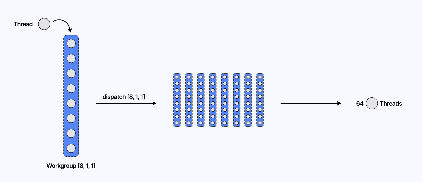
Passing this extra argument tells WebGPU how many threads/shader invocations belong to one workgroup and has the following characteristics:

• This argument has the format [x, y, z] where x, y, and z are the dimensions of the workgroup in each direction of a 3D grid.

• You can get the total number of threads per workgroup by multiplying each of x, y, and z. For example, [64, 1, 1] and [8, 8, 1] both define our workgroup of 64 threads.

• The dimensionality of the workgroup depends on how the compute shader is written and the shape of your data/buffers. For 1D buffers, [64, 1, 1] is a natural choice, whereas for 2D buffers, such as a texture, defining it as [8, 8, 1] may be more suitable.

• There is a maximum limit of 256 threads per workgroup. You can try setting [512, 1, 1], and all you'd get would be a warning from WebGPU.

• In Three.js, it is set by default to [64, 1, 1 ] ⁷.

Thus, in our previous demo, considering COUNT = 1024 instances, we would need to launch 1024 / 64 = 16 workgroups. More generally, the number of workgroups is ceil(COUNT / workgroupSize.x) in the 1D case.

Now there is also a "secret third thing" called the dispatch size. By default, when using the .compute method, you don't have to worry about it, as TSL/Three computes a dispatch size for you from count and the given (or default) workgroup size ⁸

If, however, you want to employ a more manual approach to know how many workgroups to launch, you can set it up manually using the .computeKernel method instead, which was recently added to the Three.js codebase.

In our case, since we have 1024 instances:

• We could use a dispatch size of [16, 1, 1], which would result in creating 1024 threads (64 * 16 * 1 * 1 * 1 * 1), one for each instance, which would be enough for our use case.

• For a 2D dimensionality, we could define it as [8, 8, 1] with a workgroup size of [4, 4, 1] which would give us  4 * 8 * 4 * 8 * 1 * 1 = 1024

In a nutshell:

• workgroupSize is the number of threads per workgroup.

• dispatchSize is the number of workgroups per dimension.

• Total threads = (workgroupSize.x * dispatchSize.x) × (workgroupSize.y * dispatchSize.y) × (workgroupSize.z * dispatchSize.z).

We won't use dispatch size in any examples, but I thought it was important to mention it as it informs us of the inner workings of the compute pipeline.

In the first parts of this article, we walked through the basics of WebGPU/TSL and its Node System while exploring the potential of compute shaders for our 3D work. Using them alongside instancedMesh is only one of the many use cases for compute shaders, and I wanted to dedicate the following sections of this article to more practical examples that could not only fill the blanks when it comes to porting specific work to TSL, but also be good candidates to leverage the compute pipeline.

The first practical use case that I found interesting and that showcased many benefits after porting them to TSL and making them use compute shaders is particles.

In 2022, I wrote an article covering many aspects of particles. Among those, my favorite one was GPGPU particles. Back then, we were using a Frame Buffer Object (FBO) to render in a texture off-screen filled with the position data of each particle on a given frame. After updating each of those positions via a fragment shader, we would then pass the resulting texture to the final shader to get the new positions and render the particles.

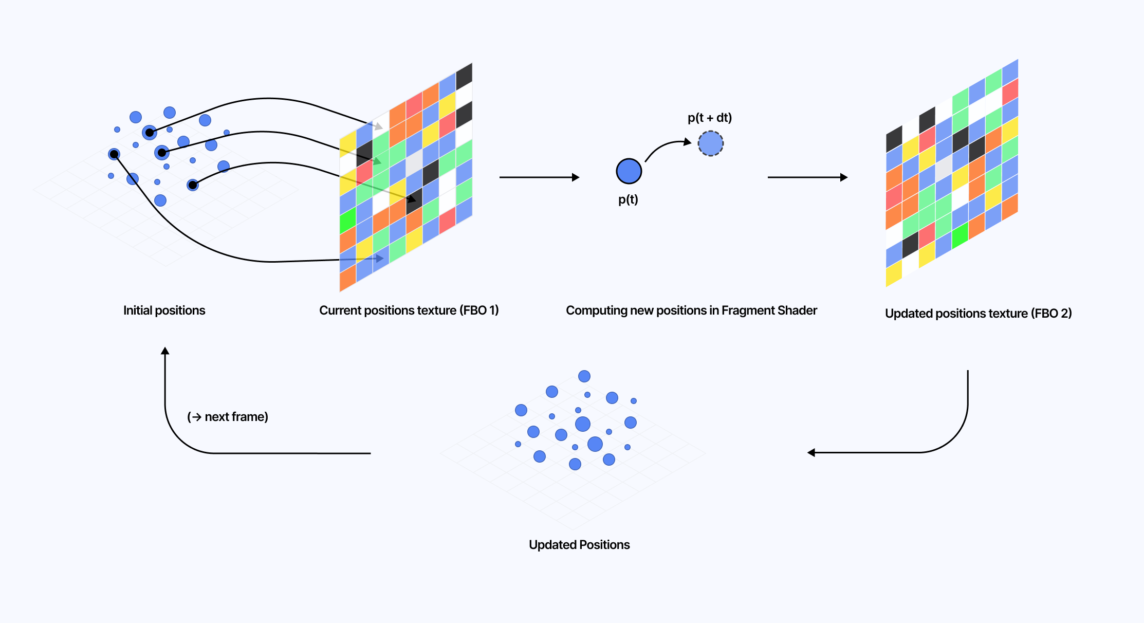
Today, all of that can be moved to the compute shader! Not only the position update, but also the instantiation of the particles themselves, which historically we've always done on the CPU.

Setting up our Particle System with Compute Shaders

Let's start by setting up a scene that demonstrates how to instantiate a particle system using the compute pipeline.

We will use sprite as our "mesh" for particles, alongside the material it pairs with: spriteNodeMaterial. Akin to instancedMesh, this construct takes a count prop, which corresponds to the number of particles we wish to render on screen. Its node material can take many of the properties we've already covered in this article, such as positionNode or colorNode, allowing us to customize our particle system with shaders.

If we were to render this as is, all the particles would render at (0, 0, 0). We can set up an instancedArray of vec3 that will hold all the initial positions for our particles. Then, we can use a compute shader that we'll dub computeInit to initialize the particles at the desired position in that buffer.

In the code snippet above:

1. We initialize all the positions of our particles randomly within a sphere of radius 2. The storage buffer for our particles will get filled at render time.

2. We then resolve and pass the position vector of each particle of a given instance via the positionNode of our spriteNodeMaterial and by leveraging instanceIndex.

Attractors with Compute Shaders

With the initialization alone, we already have a good use case for using the compute pipeline: what used to be done on the CPU is now performed on the GPU. However, we can do better!

In the case of GPGPU particles, we can replace the entire FBO and texture writing process with a single compute shader that we run on every frame. This grandly simplifies the implementation of a particle system where the position of a particle at time t depends on its previous position at a time t - dt, i.e., defined through a parametric equation such as Attractors.

Here, we will add an extra storage buffer called offsetPosition that will contain all the positions of our particles at a given frame. These offset positions will continuously update based on their previous values as we call the compute shader to fill them on every frame.

We can then get the offset position of a given instance using instanceIndex and add it to its corresponding spawn position. The diagram below illustrates this example of a compute pipeline running on every frame to update a particle system:

As for the scene itself, the demo that follows combines the compute shader used to instantiate our particle system with the one that updates their position over time. In this specific case, the attractorFunction represents a Thomas Attractor.

As someone who's quite fond of post-processing, I was disappointed to find out that effects with TSL weren't as documented as I would have thought, making porting scenes from standard React Three Fiber using @react-three/postprocessing a bit tricky at first. I had to look at a couple of examples from the Three.js examples repository and figure out through trial and error how to make them work on top of my existing React Three Fiber setup.

This section aims to make this migration a bit easier for people getting started, while also providing a practical case for compute shaders with post-processing effects.

Setting up custom post-processing effects with TSL on React Three Fiber

Similar to what we established in the second part of this article, I also like to organize my post-processing-related TSL node inside useMemo. TSL provides a few helper functions we're going to use to set up our post-processing pipeline:

• pass, which is the node that creates a new render pass ⁹

• getTexture, a method from PassNode that returns the texture for a given output name. By default, it can return either the diffuse texture or the depth texture.

• setMRT, a method from PassNode that allows you to reference additional render targets (hence the MRT -> Multiple Render Targets name)

Then we need to:

1. Create a new instance of THREE.PostProcessing against our WebGPU renderer.

2. Set its ouputNode property to any pass we want, as well as save the resulting instance to a React ref for later reference.

3. Call the render method of our post-processing instance.

The tricky part was to figure out where to call render in the first place. I knew it would be within useFrame, but at first glance, that did nothing. To make this work, we need to set the renderPriority argument of useFrame to 1. Doing so has the following effect:

• It disables React Three Fiber's automatic rendering.

• It will execute our post-processing useFrame after any other useFrame we may have ¹⁰ and thus ensure the underlying scene is fully rendered before our post-processing pipeline takes effect.

We can now create a custom post-processing pass that can be implemented with TSL or WGSL/GLSL shaders (whichever we may like). Here's the boilerplate code that I've used in my work:

The code snippet above can be used as a starting point for your own post-processing work. Here, our effect shader increases the red color channel of the input texture, which should result in a tinted scene if everything is set up correctly.

Post-processing effects with Compute Shaders

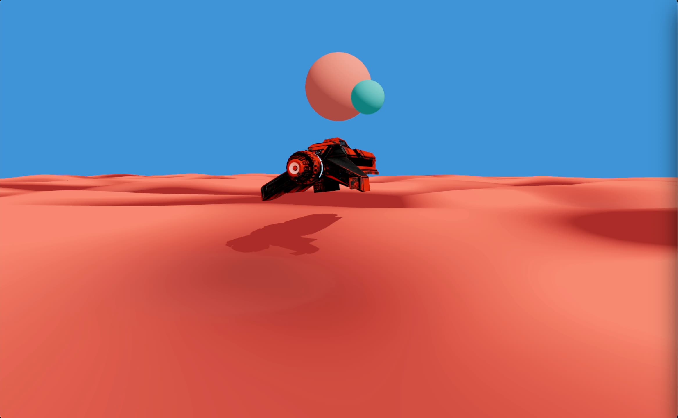
Now that we know how to work with post-processing on React Three Fiber with TSL, let's build an example that leverages the compute pipeline alongside a custom shader effect to stylize our scene. For this section, we'll reimplement the outline effect I introduced in Moebius-style post-processing and other stylized shaders that is based on an edge detection filter called "Sobel filter".

As a reminder, to get our edge detection filter working, we will first need:

• The depth texture of the scene. This will inform us of sharp differences in depth where we'd want to draw outlines to differentiate foreground and background.

• The normal texture of the scene. This will inform us of any sharp changes of direction for any mesh in our scene. Likewise, we want to draw outlines to highlight the details within a mesh.

Diagram showcasing how combining the outputs of the Sobel filters for both Depth and Normal data gives us the outlines for the entire scene and each meshes within it

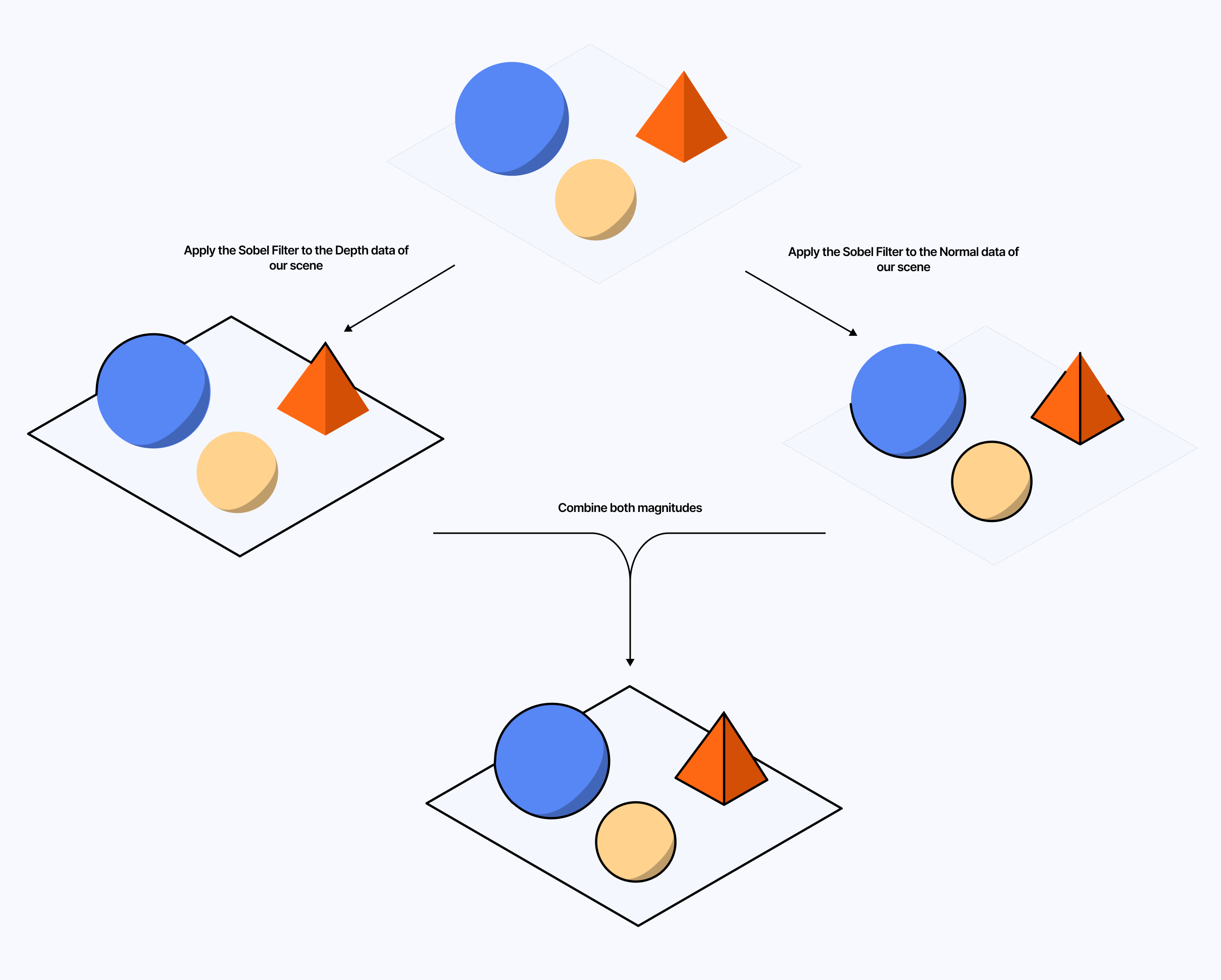
The combination of both rates of change/gradients (normal and depth) gives us an overall magnitude of change, i.e., the strength of an edge at a given position on the screen. We can then correlate this strength to either the intensity or the thickness of the outline.

In my original write-up on the topic, I did those calculations directly in the final effect. Today, though, we can:

1. Leverage a compute shader to fill a StorageTexture with the magnitude at each UV.

2. Pass this StorageTexture as an argument to our final effect, which is now only responsible for interpreting that data to draw the final outlines.

3. Call our compute shader once or on every frame if the scene is dynamic.

In the compute phase:

• We set up and pass a THREE.StorageTexture with a size matching our screen's size.

• We had to calculate the x and y coordinates by converting our instanceIndex into 2D pixel coordinates using the dimensions of our texture.

• From those, we could also infer our UV coordinates, which are necessary to compute the depth and normal magnitudes.

• Once we have calculated the overall magnitude, we can then write to the texture using the textureStore TSL function.

We will then have to set up our compute shader to create one thread per pixel of our screen, i.e. window.innerWidth * window.devicePixelRatio * window.innerHeight * window.devicePixelRatio. We can then call it using gl.compute in our useFrame, thus ensuring it updates the texture containing our magnitude data on every frame to handle any camera angle change or any mesh movement.

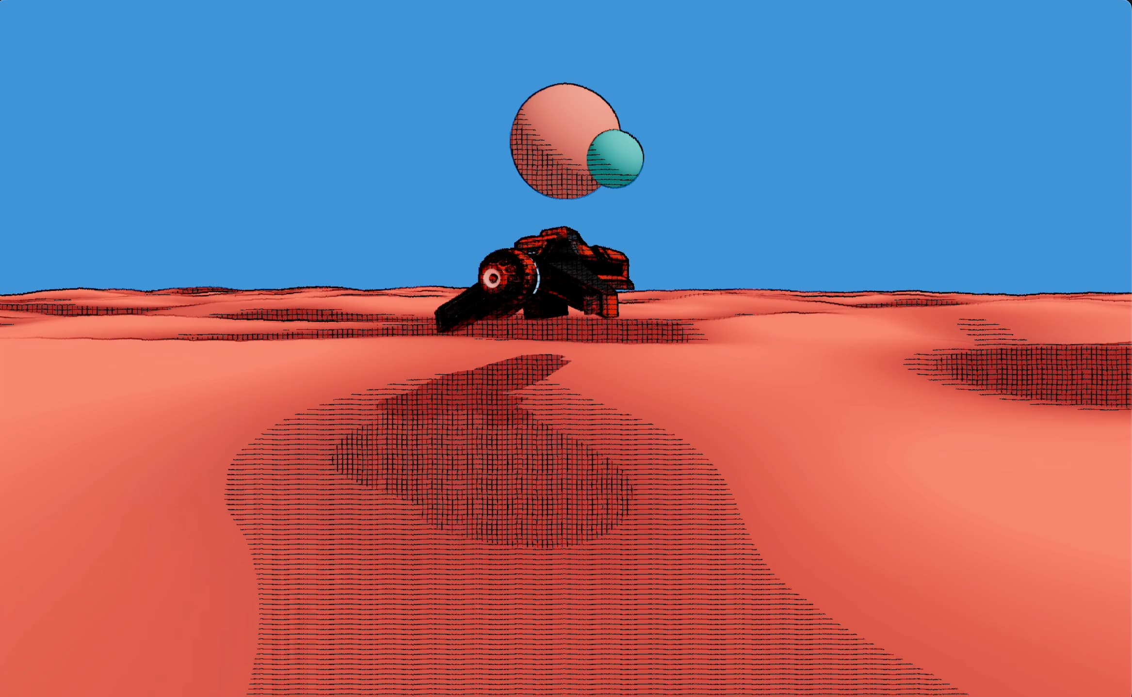
The demo below contains the combination of:

• our compute pipeline, running our Sobel filter and storing the resulting magnitudes in a texture.

• our render pipeline, running our scene, and applying our custom outline effect based on the magnitude data stored in the texture.

I could have written a standalone article for each of the examples and themes presented in this post. However, it felt more natural to showcase them together so that it could act as a guide for anyone looking to transition from classic Three.js/React Three Fiber to this new way to build 3D for the web. I hope this answers some of the questions you may have had regarding WebGPU and TSL, and provides clarity on aspects that may not be immediately apparent from the available documentation and examples.

If I had to write down a couple of my own thoughts at this point in my learning journey, they would be the following:

1. The node system is life-changing. I really like it. I think many other developers will agree with me on this one.

2. TSL abstracts a lot of things away, which is both good, as it is very friendly to beginners and lowers the barrier of entry for shader development, but can also be a hassle sometimes as we're giving up control for more advanced use cases.

3. The abstraction of TSL, while being great for working fast and focusing on building, may prompt me to start working with WebGPU outside of the framework of Three.js/React Three Fiber. There are projects like TypeGPU that make working with WebGPU more accessible while not completely hiding its core features away from developers.

4. TSL still is very much a Work In Progress, many of its features are loosely or not documented at all. This is where the majority of my frustration with it lies. I often found myself having to infer the usage of a function or to dig an example somewhere within the Three.js repository, which slowed me down in my work. I'd love a full specification to be written at some point so it can remove the guesswork from using it and document best practices to follow.

In the meantime, as some of those details get ironed out, I will still be writing shaders in GLSL unless I have a specific use case where I'd need compute shaders, like in my recent procedural landscape experiences, which I'm very excited to tell you more about the day this project is ready. If you need more inspiration to apply your newly acquired TSL/WebGPU knowledge, here's the list of all the other scenes I built over the summer. You can try to reproduce these on your own to get even more comfortable with TSL and WebGPU; everything you need was introduced in this article:

1. WebGPU WebKit for Safari 26.0 adds support for WebGPU.

2. A comparison of Performance on WebGPU and WebGL in the Godot game engine

3. It also depends on whether you use compute shaders or not since they are a WebGPU only feature

4. Async GL prop - React Three Fiber docs

5. WebGPU Uniforms - WebgpuFundamentals.org

6. WebGPU API - MDN

7. https://github.com/Spiri0/three.js/blob/aa60b0cca42da40b489070a135d4a23459bad59e/src/nodes/gpgpu/ComputeNode.js#L214

8. https://github.com/Spiri0/three.js/blob/aa60b0cca42da40b489070a135d4a23459bad59e/src/renderers/webgpu/WebGPUBackend.js#L1356-L1387

9. https://github.com/mrdoob/three.js/blob/9e7a65c17bc3832798103190df8f674b9acca073/src/nodes/display/PassNode.js#L162

10. Taking over the render-loop - React Three Fiber docs