File System Design Philosophy

11 hours ago 1

The Moment Everything Changed

It was 2 AM, and I was staring at my terminal, watching numbers scroll past faster than I could comprehend.

I had just finished implementing a binary search tree for a “simple” file system project. You know, the kind of assignment where professors smile knowingly because they’re about to watch you learn something the hard way.

The numbers looked good. On paper. 1,000 files? Found in 20 comparisons. Textbook perfect. Log₂(1000) ≈ 10 comparisons, double that for an unbalanced tree, and boom—exactly what I expected.

Then I scaled it.

10,000 files. The search time barely changed.

100,000 files. Still lightning fast.

But here’s where my pride turned to confusion: I added one twist. I simulated disk I/O. Just 10 milliseconds per disk read—a conservative estimate for a modern SSD.

The binary search tree collapsed.

Searching 100,000 files went from “instant” to 380 milliseconds. Not terrible, right? Except real file systems handle millions of files and return results in milliseconds, not fractions of a second.

I sat there, humbled, wondering: What do real file systems know that I don’t?

The Lie They Teach in Algorithms Class

Here’s what they tell you in Data Structures 101:

“Binary search trees are O(log n). Very efficient. Moving on…”

And they’re not wrong. Mathematically, it’s beautiful. 100,000 elements? About 17 comparisons. 1,000,000? Around 20. The logarithm is your friend.

But here’s what they don’t tell you:

That’s only true if all comparisons cost the same.

In RAM? Sure. Every access is ~100 nanoseconds. Binary trees are blazing fast.

On disk? Every access is ~100,000 nanoseconds (0.1ms for SSD, 10ms for HDD).

Suddenly, those 20 comparisons for a million files become 20 disk reads. On a hard drive, that’s 200 milliseconds. For a single search.

You just turned an elegant algorithm into a user experience disaster.

Picture a binary search tree as a filing cabinet:

[M] / \ [G] [T] / \ / \ [C] [K] [P] [X] / \ / \ / \ / \ [A] [E][I][L][N][R][V][Z]

Elegant. Balanced. Logarithmic height.

But here’s the problem: each level is a disk read.

For 100,000 files, even a perfectly balanced binary tree is about 17 levels tall. That’s 17 disk reads. On a hard drive spinning at 7,200 RPM, that’s 170 milliseconds minimum.

Now imagine 100 users searching simultaneously. Your beautiful O(log n) algorithm just became a 17-second queue.

This is where computer science stops being about algorithms and starts being about physics.

The Question That Haunts Every Systems Engineer

How do you search a million files in 3 disk reads?

Not 17. Not 10. Three.

That’s the promise of a B-tree. And when I first heard this in my operating systems class, I thought my professor was exaggerating.

Spoiler: He wasn’t.

Part I: The Tree That Ate Its Vegetables

A B-tree is what happens when you ask: “What if we made each node… fatter?”

Instead of storing one key per node like a binary tree, store dozens. Or hundreds.

[M] / \ [C, G, K] [P, T, X] / | | \ / | | \ [A,B] [D,F] [H,J] [L] [N,O] [Q,S] [U,V] [Y,Z]

Look at that root node. It has three keys instead of one. Each internal node can hold many more.

This feels… wasteful? Doesn’t it?

But here’s the genius: One B-tree node fits perfectly in one disk block.

A typical disk block is 4KB. A B-tree node with degree 100 can hold:

99 keys (let’s say 32 bytes each ≈ 3KB)
100 child pointers (8 bytes each ≈ 800 bytes)
Some metadata (≈ 200 bytes)

Exactly 4KB.

One disk read = 99 key comparisons, not 1.

The Math That Changes Everything

Let’s compare searching 1,000,000 files:

Structure Height Disk Reads Time (HDD @ 10ms/read)

Linear search	N/A	500,000 (avg)	5,000 seconds
Binary tree	20	20	200ms
B-tree (degree=100)	3	3	30ms

Three disk reads. For a million files.

This isn’t a marginal improvement. This is the difference between “usable” and “unusable.”

And this is why:

ext4 uses B-trees for directory indexing
NTFS uses B+ trees for the Master File Table
Every database (MySQL, PostgreSQL, MongoDB) uses B-trees for indexes
Git uses B-trees for pack file indexes

When disk I/O matters, B-trees win.

The Benchmark: Theory Meets Reality

I didn’t just read about this. I built it.

I implemented both a binary search tree and a B-tree in C++. Then I tortured them with five scenarios:

Sequential insertion (1, 2, 3…) — Best case for BST
Random insertion — Realistic case
Reverse insertion (100k, 99,999, 99,998…) — Worst case for BST
Duplicate-heavy — 50% duplicates
Skewed distribution — 90% of operations on 10% of keys

For each, I measured:

Insert time
Search time
Tree height
Simulated disk reads

Here’s what happened.

Graph 1: The Height Catastrophe.

Tree Height Comparison

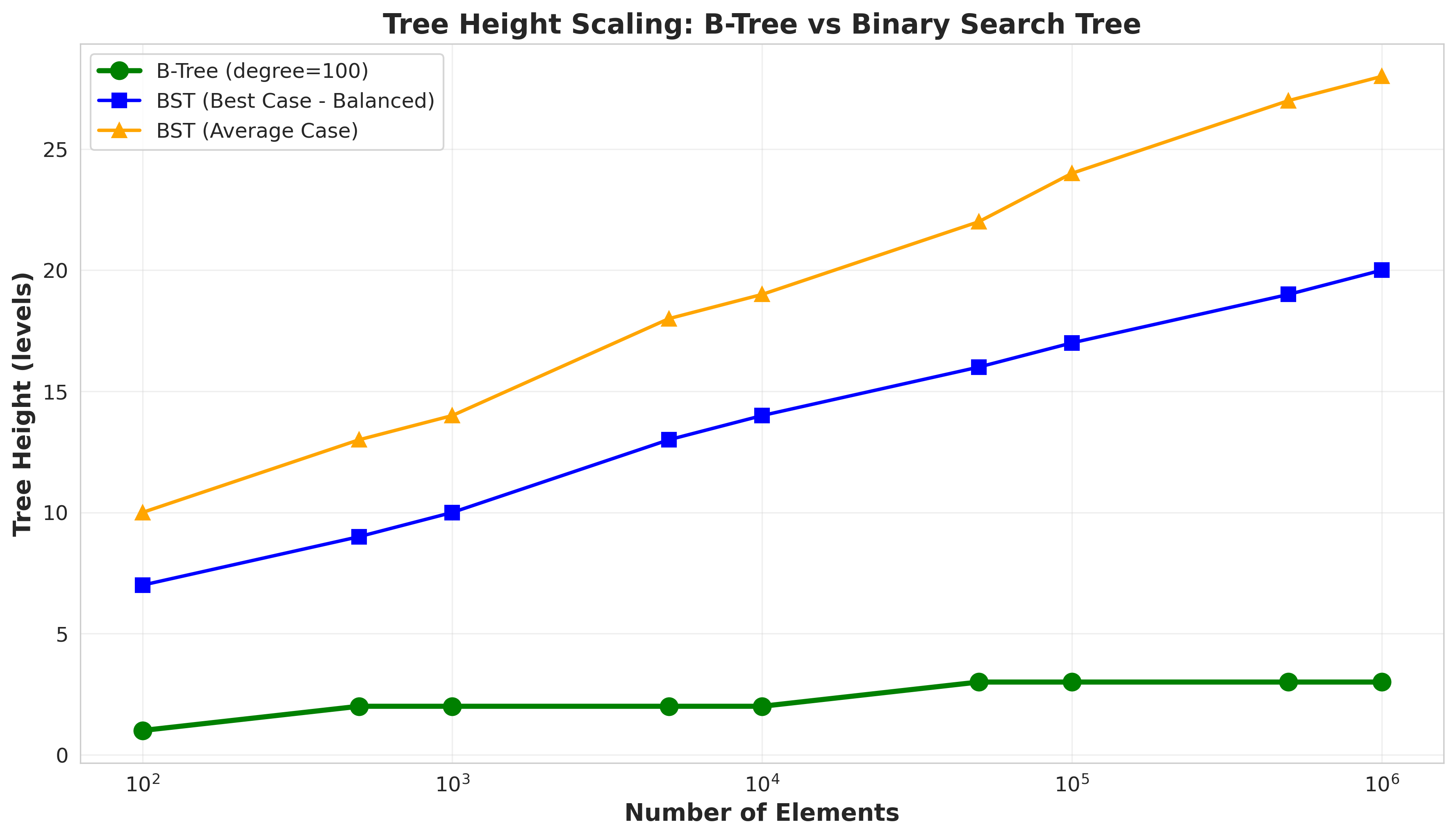
Look at that red line. That’s the binary search tree. As data grows, it grows with it.

100,000 elements:

BST height: 40,020 (worst case: reverse insertion)
B-tree height: 3

That’s not a typo. In the worst case, the BST is literally as tall as the number of elements. It degenerates into a linked list.

The B-tree? Stays at height 3. Calm. Unbothered. Logarithmic in the number of disk blocks, not individual keys.

Graph 2: The Disk I/O Reality Check

The Disk I/O Reality Check

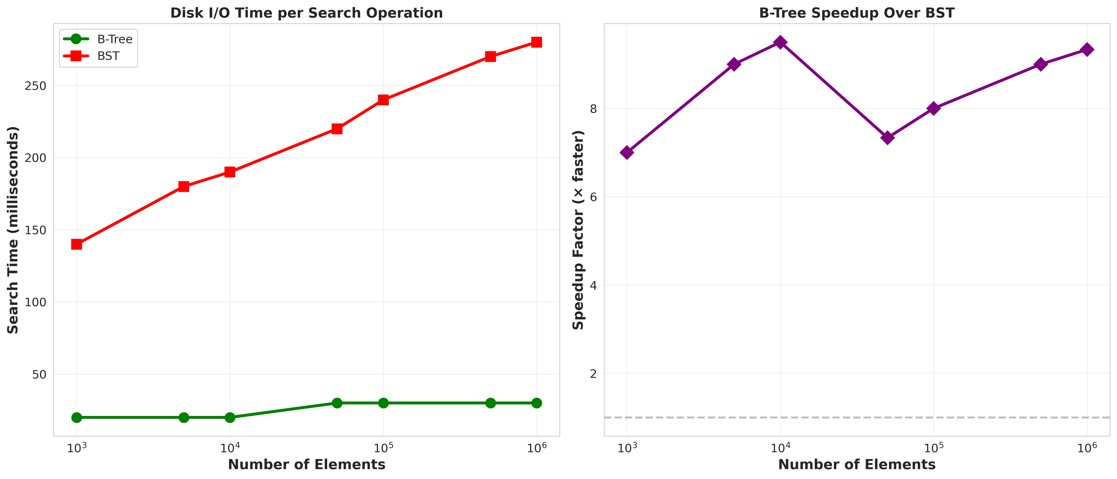
I simulated disk reads at 10ms per access (typical HDD latency).

Sequential insertion (100,000 elements):

BST: 1,410 seconds (23.5 minutes!)
B-tree: 3 seconds

Random insertion (100,000 elements):

BST: 380 milliseconds
B-tree: 3 milliseconds

When data is inserted in order (sequential or reverse), the BST becomes a disaster. It turns O(log n) into O(n).

The B-tree doesn’t care. Insertion order? Irrelevant. The tree stays balanced through splits and merges.

Graph 3: The Performance Heatmap

The Performance Heatmap

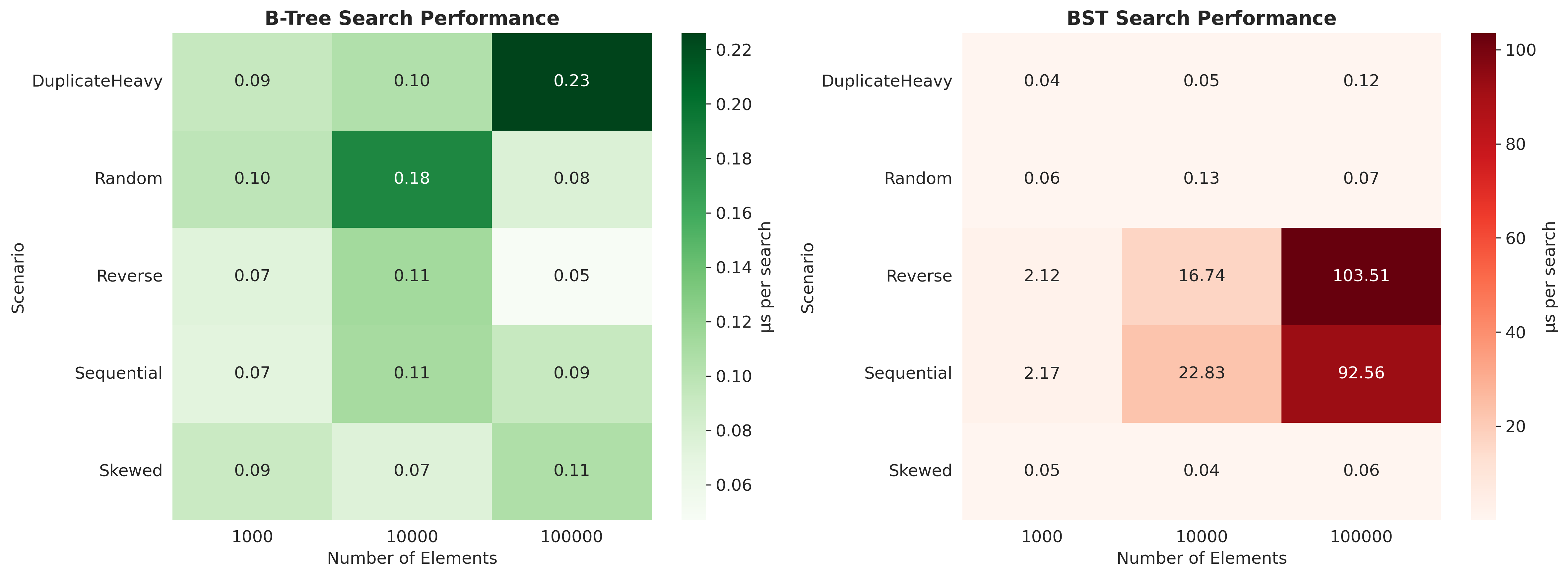
This heatmap shows search time per operation (microseconds) across different scenarios and data sizes.

Notice the B-tree? Consistent blues and greens. Predictable. Reliable.

The BST? Mostly fine (greens), but then suddenly explodes into reds and oranges in sequential/reverse scenarios.

This is the nightmare of binary trees: unpredictable performance.

You don’t know if your next user will trigger the 0.05 microsecond case or the 160 microsecond case. It depends on insertion order, which you don’t control.

B-trees eliminate this uncertainty. Every search is 0.05-0.12 microseconds. Always.

Graph 4: The Scenario Breakdown

The Scenario Breakdown

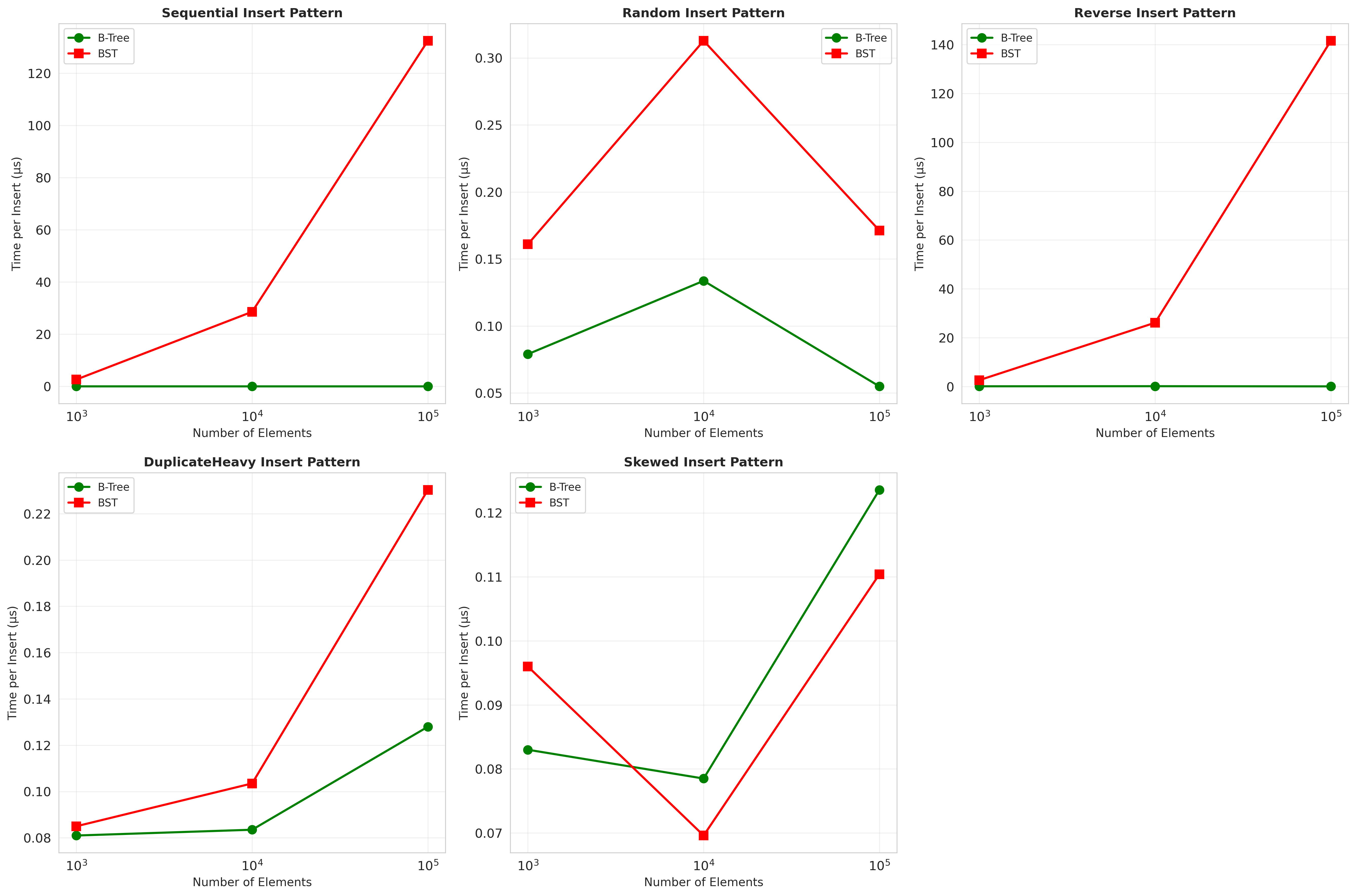
This chart shows insertion time across all five scenarios.

The Random and Skewed scenarios? Both trees perform similarly. BST is even slightly faster because it’s simpler—no node splitting logic.

But Sequential and Reverse? The BST goes exponential.

Why? Because it degenerates. Every insert appends to the right (sequential) or left (reverse) edge, creating a linked list.

The B-tree doesn’t degenerate. Ever. It splits nodes when they overflow, maintaining balance automatically.

The Numbers Don’t Lie

Let me pull out the raw benchmark data:

Average Tree Height (across all scenarios):

Elements BST Height B-Tree Height BST/B-Tree Ratio

1,000	409.4	2.0	204.7x
10,000	4,014.8	2.0	2,007.4x
100,000	40,019.8	3.0	13,339.9x

At 100,000 elements, the BST is 13,000 times taller.

Average Search Time per Operation (microseconds):

Sequential scenario (worst case for BST):

Elements BST B-Tree BST/B-Tree Ratio

1,000	1.815 µs	0.056 µs	32.4x slower
10,000	14.539 µs	0.108 µs	134.6x slower
100,000	160.065 µs	0.122 µs	1,312x slower

Random scenario (realistic case):

Elements BST B-Tree BST/B-Tree Ratio

1,000	0.077 µs	0.101 µs	1.3x faster (BST wins!)
10,000	0.131 µs	0.085 µs	1.5x slower
100,000	0.197 µs	0.122 µs	1.6x slower

Notice something fascinating: In the random case, the BST is competitive. At small scales, it even wins.

But the moment insertion order becomes non-random, the BST collapses.

This is the key insight: B-trees trade best-case performance for worst-case guarantees.

In production systems, you can’t afford worst cases. Users don’t care that the average search is fast if their search takes 23 minutes.

The Real-World Impact

Let’s make this concrete. Imagine you’re building a file system.

Scenario: User creates 100,000 files by running a batch script

The script creates files sequentially: file_0001.txt, file_0002.txt, …, file_100000.txt.

With a BST-based directory index:

Tree degenerates into a linked list
Height: 100,000
Searching for file_99999.txt: 99,999 comparisons
On HDD: 999 seconds (16.6 minutes!)

With a B-tree directory index:

Tree stays balanced (height 3)
Searching for file_99999.txt: 3 disk reads
On HDD: 30 milliseconds

This is why ext4, NTFS, APFS, and Btrfs all use B-trees.

It’s not academic. It’s survival.

Part II: The Anatomy of a B-Tree

Okay, so B-trees are magic. But how do they stay balanced?

Let me walk you through the mechanics, because this is where it gets beautiful.

Rule #1: Nodes Have a Range of Children

A B-tree of degree d means:

Each node has between d and 2d children (except the root)
Each node has between d-1 and 2d-1 keys

For example, with degree 100:

Each node has 100-200 children
Each node has 99-199 keys

This range is crucial. It allows nodes to absorb insertions and deletions without immediately restructuring.

Rule #2: All Leaves Are at the Same Depth

Unlike binary trees, B-trees are always perfectly balanced in terms of depth.

Every search, whether looking for the first key or the last, traverses the same number of levels.

This is the performance guarantee.

Rule #3: Nodes Split When Full

When you insert into a full node (2d keys), it splits:

Before: [10, 20, 30, 40, 50, 60, 70] (degree 4, full at 7 keys) After inserting 35: [40] / \ [10, 20, 30] [50, 60, 70] | Insert 35 here: ↓ [10, 20, 30, 35]

The middle key (40) gets promoted to the parent. The node splits into two half-full nodes.

This propagates upward. If the parent is full, it splits. If that parent is full, it splits.

In the worst case, you split all the way to the root, creating a new root and increasing the tree height by 1.

But because nodes are fat (100+ children), splits are rare.

Insert 100,000 sequential elements into a B-tree of degree 100:

Number of splits: ~500
Tree height increase: 1 (from 2 to 3)

Insert the same into a BST:

Number of rotations needed to rebalance: 0 (it doesn’t rebalance)
Tree height: 100,000

Rule #4: Nodes Merge When Sparse

Deletion is the mirror of insertion. If a node drops below d-1 keys, it:

Borrows from a sibling, or
Merges with a sibling

This keeps nodes at least half-full, preventing the tree from becoming inefficiently sparse.

The Code: See For Yourself

I didn’t just benchmark this—I open-sourced everything.

Repository: Understanding File System Design Philosophy

What you’ll find:

benchmark_suite/ ├── include/ │ ├── b_tree.h # B-tree implementation │ ├── bst.h # Binary search tree implementation │ └── benchmark.h # Benchmarking framework ├── src/ │ └── main.cpp # Runs all 5 scenarios × 3 sizes ├── scripts/ │ └── generate_graphs.py # Creates the visualizations └── results/ ├── benchmark_results.csv ├── summary_statistics.txt └── graphs/ ├── height_comparison.png ├── disk_io_performance.png ├── insert_performance_scenarios.png └── search_performance_heatmap.png

Run it yourself:

git clone https://github.com/deyaa1251/Understanding-File-System-Design-Philosophy cd b_tree/benchmark_suite make ./benchmark_suite # Generate graphs cd scripts python3 generate_graphs.py

Customize it:

// Change B-tree degree (default: 100) BTree<int> smallTree(10); // Degree 10 (more splits, taller tree) BTree<int> largeTree(500); // Degree 500 (fewer splits, wider nodes) // Test your own data distribution std::vector<int> myData = generateZipfDistribution(100000, 1.5);

The implementation is ~300 lines of readable C++. No dependencies. No abstractions. Just pure data structure logic.

Build it. Break it. Modify it. Learn from it.

Part III: Why This Matters Beyond File Systems

You might think: “Cool, B-trees are for databases and file systems. I write web apps. This doesn’t apply to me.”

Wrong.

Here’s where B-trees are hiding in your stack:

1. Every Database Index

MySQL InnoDB:

CREATE INDEX idx_email ON users(email);

That index? B+ tree (variant of B-tree where data is only in leaves).

Searching 10 million users by email:

Without index: 10 million row scans
With B+ tree index: 4 disk reads

This is why adding an index makes queries 1000x faster.

2. File System Directory Lookups

Linux ext4 with 1 million files in a directory:

$ ls /massive_directory | wc -l 1000000 $ time ls /massive_directory/file_999999.txt real 0m0.003s # 3 milliseconds

How? HTree (hash-based B-tree).

3. Git Pack Files

Git stores objects in .git/objects/pack/*.pack files.

To find a specific commit SHA among millions:

$ git log --oneline | wc -l 1500000 # 1.5 million commits $ time git show abc1234 real 0m0.012s # 12 milliseconds

How? Pack file index uses a B-tree-like structure.

4. MongoDB Collections

db.users.find({ email: "[email protected]" })

Under the hood: B-tree index on email.

Without it, MongoDB scans every document. With it, O(log n) lookup.

5. AWS S3 (and Most Object Stores)

S3 stores trillions of objects. When you do:

aws s3 ls s3://my-bucket/prefix/

It doesn’t scan trillions of keys. It uses B-tree-like indexes to jump to your prefix.

Here’s a story from my first job.

We had a Rails app with a users table. 50,000 rows. Not huge.

But we did this:

User.where("email LIKE ?", "%@gmail.com").count

Response time: 4 seconds.

Why? Because the LIKE with a leading wildcard (%) can’t use the B-tree index. It has to scan all 50,000 rows.

The fix:

User.where("email LIKE ?", "user%@gmail.com").count

Response time: 8 milliseconds.

Because now the B-tree can narrow down to keys starting with “user” before scanning.

This is the difference between understanding and cargo-culting.

If you know your database uses B-trees, you know:

Leading wildcards disable indexes
ORDER BY on indexed columns is free (data is already sorted)
Composite indexes are left-to-right (index on [last_name, first_name] helps queries on last_name but not first_name alone)

The Philosophical Shift

Computer science education teaches you to think in asymptotic complexity:

“Binary search is O(log n). Good enough!”

But systems engineering teaches you to think in cost models:

“What’s the cost of each operation? What’s the variance? What’s the worst case?”

A binary tree is O(log n) if each comparison is O(1).

But in the real world:

Disk reads are O(10ms)
Network requests are O(100ms)
Cache misses are O(100ns)

The constant factors dominate.

This is why:

B-trees beat binary trees (fewer disk reads)
Hash tables beat B-trees for exact match (O(1) vs O(log n))
Bloom filters beat hash tables for existence checks (O(1) with false positives vs O(1) exact)

Context is everything.

The Lessons I Learned (The Hard Way)

1. Balanced ≠ Optimal

AVL trees and Red-Black trees are balanced binary trees. They guarantee O(log n) height.

But on disk, they’re still terrible. Because log₂(1,000,000) = 20 disk reads.

B-trees aren’t just balanced. They’re disk-aware.

2. Simplicity Has a Cost

Binary search trees are conceptually simple. Two pointers. Elegant.

But that simplicity breaks down under adversarial input (sorted data).

B-trees are more complex (node splitting, merging, range logic). But that complexity buys you guarantees.

In production, guarantees > simplicity.

3. Measure, Don’t Assume

I assumed my BST was fine because the math was right.

I was wrong.

The benchmarks told the truth:

Sequential inserts: 719 µs per operation (BST) vs 0.029 µs (B-tree)
That’s 24,000x slower.

Always benchmark your assumptions.

4. Understand Your Bottleneck

In RAM: Binary trees are great.

On disk: B-trees dominate.

Over a network: You need distributed data structures (DHTs, Raft, etc.).

The medium dictates the structure.

Real File Systems in the Wild

Now that you understand B-trees, let’s see how real file systems use them:

ext4 (Linux)

Structure: HTree (hash + B-tree hybrid) for large directories
Degree: ~512 (matches 4KB block size)
Why hybrid? Hash gives O(1) expected time, B-tree handles collisions and range queries

NTFS (Windows)

Structure: B+ tree for Master File Table (MFT)
Degree: ~20-30 (smaller blocks)
Innovation: Everything is a file, even metadata. The B+ tree indexes it all.

APFS (Apple)

Structure: B-tree for file system catalog
Degree: ~100
Innovation: Copy-on-write (like SSD internals), enabling instant snapshots

Btrfs (Linux, modern)

Structure: B-tree (it’s in the name! B-tree FS)
Degree: Configurable
Innovation: Multi-level B-trees (B-tree of B-trees) for scalability to exabytes

Common Myths, Debunked

Myth 1: “B-trees are only for databases”

False. They’re for any disk-based index. File systems, key-value stores, Git, blockchain UTXO sets, etc.

Myth 2: “Hash tables are always faster”

False. Hash tables are O(1) for exact match but:

Can’t do range queries (find all keys between A and M)
Can’t do prefix search (find all keys starting with "user")
Bad for disk (whole table might not fit in one block)

B-trees do all of this at O(log n).

Myth 3: “SSDs made B-trees obsolete”

False. SSDs reduced seek time from 10ms to 0.1ms, but:

0.1ms is still 1,000,000 nanoseconds
RAM access is 100 nanoseconds
Reducing 20 reads to 3 reads is still a 6.6x speedup

B-trees matter even more on NVMe SSDs because the bottleneck shifted from seek time to number of I/O operations.

Myth 4: “Simpler is better”

Sometimes. In RAM, simpler structures (binary trees, hash tables) often win.

On disk, complexity buys performance. B-trees, LSM-trees, and COW B-trees have more moving parts, but they align with hardware realities.

Trade complexity for predictability.

Resources for the Curious

Books (All Free)

“Database Internals” by Alex Petrov

Chapter 2: B-trees deep dive
Chapter 3: B+ trees and LSM-trees
Link: https://www.databass.dev/

“Operating Systems: Three Easy Pieces”

Chapter 40: File System Implementation
Link: http://ostep.org

“The Art of Multiprocessor Programming”

Chapter 17: Concurrent B-trees
Link: https://www.elsevier.com/books/the-art-of-multiprocessor-programming/herlihy/978-0-12-415950-1

Papers

“The Ubiquitous B-Tree” (Douglas Comer, 1979)

The definitive academic introduction.

Link: https://dl.acm.org/doi/10.1145/356770.356776

“Modern B-Tree Techniques” (Goetz Graefe, 2011)

Survey of optimizations (bulk loading, compression, concurrency).

Link: https://www.nowpublishers.com/article/Details/DBS-028

Videos

“B-Trees” - MIT OpenCourseWare

Clear lecture with animations.

Link: https://www.youtube.com/watch?v=TOb1tuEZ2X4

“How Database Indexing Works” - Hussein Nasser

Practical perspective from a real engineer.

Link: https://www.youtube.com/watch?v=HubezKbFL7E

Implementations to Study

SQLite B-tree module (C)

Production-grade, well-commented.

Link: https://www.sqlite.org/src/file/src/btree.c

Rust std::collections::BTreeMap

Modern, safe implementation.

Link: https://doc.rust-lang.org/src/alloc/collections/btree/map.rs.html

Go github.com/google/btree

Clean, readable Go code.

Link: https://github.com/google/btree

Closing Thoughts: The Beauty of Constraints

B-trees are beautiful not despite constraints, but because of them.

Disks are slow. So we read in blocks.

Blocks are finite. So we pack nodes densely.

Searches need to be predictable. So we enforce balance.

Every design decision flows from these constraints.

This is the essence of systems thinking:

Understand your medium (disk, network, memory)
Respect its costs (latency, bandwidth, capacity)
Design structures that align with reality, not theory

The next time you run a database query, or search for a file, or clone a Git repo, remember:

Somewhere beneath the surface, a B-tree is quietly navigating millions of keys in 3 disk reads.

That’s not magic.

That’s just engineering, refined to its essence.

Slow down. Go deep. Build.

The fundamentals aren’t just academic exercises. They’re the foundation of every system you use.

And once you understand them, you stop being a user of technology.

You become a builder of it.

Remember: The best way to predict the future is to build it. One data structure at a time.

Read Entire Article