Hopefully the Most Gentle Introduction to Simulation

A good portion of this content was originally the first set of notes for a course I took, called Topics in Computer Graphics: Seminar on Physics Based Animation mainly as an excercise to remind myself of the basic ideas when I was taking the course. I would credit a lot of this content to the course.

Arguably the primary areas of computer graphics are,

• modelling: geometric and appearance properties to store on computers
• rendering: modelling how light interacts with the world and making images
• animation: concerned with motion

But animation is not always just motion; it could also be, for instance, sound. In general, we somehow need to find ways to generate complex motions from simple rules.

Simulation or physics-based animation (atleast for the purpose of this article) has a very interesting goal: to predict the future or past of a system based on the current state of the system, so if we know some initial state of the system fully and we know the law that it satisfies we can predict the future or past.

An important distinction here is state. If you consider a particle with some motion, the future is not just defined by the the current “position” or configuration but rather it is uniquely determined by the state¹ of the system².

Before we start, a quick map of viewpoints. Newtonian, Lagrangian, and Hamiltonian are three mathematical models on the same dynamics. Newtonian talks in forces and accelerations. Lagrangian talks in energies and picks the motion that best balances them. Hamiltonian talks in positions and momenta and tracks how energy flows. Here we use the Lagrangian view because it plugs cleanly into meshes, springs, and hard constraints and turns into linear‑algebra formulas we can code. Hamiltonian has has a very nice geometric interpretation (and I actually feel this view is more natural and intuitive) and the symplectic structure is totally canonical (but they still have some of the problems of blowing up we will talk about later, after all a degree $2$ Hamiltonian gets a nonlinear ODE for momentum just like the Ricati equation which can go to $\infty$ in a finite time).

Springs are Everywhere!

When something prefers a rest shape, length, or angle and resists being changed, you can model that preference as a “spring.” In practice we attach many small, virtual springs to the parts of an object that we want to keep under control. Each spring gently pulls the system back toward a desired state; the collection of all these pulls produces realistic motion.

We can simulate cloth or deformable shapes or rigid shapes by having many-many small mass-spring systems inside the shape. After all rigidity can be seen as the limit of extremely stiff springs that forbid shape change.

Newton’s Law

Let us say we have a particle; it has a bunch of properties:

• $\color{#17becf}{x(t)}$: position in space
• $\color{#1f77b4}{v(t)} = \color{#1f77b4}{\frac{dx}{dt}} (t)$: velocity in space
• $\color{#d62728}{a(t)} = \color{#d62728}{\frac{d^2x}{dt^2}} (t)$: acceleration in space
• $\color{#7f7f7f}{m}$: mass

The momentum is $\color{#8c564b}{p} = mv$. Newton’s second law says the time rate of change of momentum $\frac{d}{dt} (mv)$ is the force $\color{#ff7f0e}{f}$. Assuming we have a constant mass, $\color{#7f7f7f}{m} \, \color{#d62728}{\frac{dv}{dt}} = \color{#ff7f0e}{f}$. This is called vectorial mechanics.

We are more interested in variational mechanics or analytical mechanics³, which is based on two fundamental energies (kinetic and potential) rather than these vector properties. Here, motion is defined using a variational principle, \begin{equation} e\big(f(t), \, \dot f(t), \ldots\big) \;\longrightarrow\; \mathbb{R}, \end{equation} where $e$ is a functional, and $f(t), \dot f(t), \ldots$ are functions of time and their derivatives.

Generalized Coordinates

One thing we need for variational mechanics is generalized coordinates⁴. $\color{#17becf}{q(t)}$ are coordinates we use in our simulation, and a function $f$ translates these into world coordinates: \begin{equation} \color{#17becf}{x(t)} = f(\color{#17becf}{q(t)}). \end{equation} We can get velocity by the chain rule⁵, \(\begin{equation} \color{#1f77b4}{\frac{dx}{dt}} (t) = \overbrace{\color{#8c564b}{\frac{df}{dq}}}^{\color{#8c564b}{\text{Jacobian}}} \underbrace{\color{#1f77b4}{\dot q(t)}}_{\color{#1f77b4}{\text{generalized velocity}}}. \end{equation}\) For example, a particle moving in space: $x(t) = q(t) \in \mathbb{R}^3$ can represent the position of the center of the particle, in which case the Jacobian is the identity. Another example is adding rigid motion: \(x(t) = \underbrace{RX + p}_{q}\), where \(\underbrace{R \in SO(3)}_{3\times 3\, \text{matrix}}\) and $p \in \mathbb{R}^3$.⁶

Lagrangian

\[\begin{equation} \underbrace{\color{#bcbd22}{L}}_{\color{#bcbd22}{\text{Lagrangian}}} = \overbrace{\color{#2ca02c}{T}}^{\color{#2ca02c}{\text{KE}}} - \underbrace{\color{#9467bd}{V}}_{\color{#9467bd}{\text{PE}}}. \end{equation}\]

Let us say we have two times and the particle passes from one to the other. Leibniz conjectured that we could find the path between them by finding a stationary point of the action⁷. The action is a functional mapping $q$ and its time derivative to a scalar value, i.e. the integral of the Lagrangian over time: \begin{equation} \color{#e377c2}{S}(q(t), \dot q(t)) = \int_{t_1}^{t_2} \big( T(q(t), \dot q(t)) - V(q(t), \dot q(t)) \big)\, dt. \end{equation} We can minimize by finding a flat spot by perturbing the trajectory and seeing whether $\color{#e377c2}{S}$ changes: \begin{equation} \color{#e377c2}{S}(q + \delta q, \dot q + \delta \dot q) = \color{#e377c2}{S}(q(t), \dot q(t)). \end{equation} Then these are the correct solutions. But how do you find $q$? This is where the calculus of variations comes in: \begin{equation} \begin{split} \color{#e377c2}{S}(q(t), \dot q(t)) &= \int_{t_1}^{t_2} L(q(t), \dot q(t))\, dt, \\\
\color{#e377c2}{S}(q + \delta q, \dot q + \delta \dot q) &= \int_{t_1}^{t_2} L(q + \delta q, \dot q + \delta \dot q)\, dt. \end{split} \end{equation} Now apply a Taylor expansion inside the integral,⁸

\[\begin{equation} \approx \underbrace{\int_{t_1}^{t_2} L(q, \dot q)\, dt}_{\color{#e377c2}{S}(q(t), \dot q(t))}\; +\; \overbrace{\int_{t_1}^{t_2} \frac{\partial L}{\partial q}\, \delta q + \frac{\partial L}{\partial \dot q}\, \delta \dot q\, dt}^{\text{First variation }\, \color{#e377c2}{\delta S}(q(t), \dot q(t))}. \end{equation}\]

So all you need to do is find $q$ for which the first variation is $0$:

\[\begin{equation} \int_{t_1}^{t_2} \frac{\partial L}{\partial q}\, \delta q + \underbrace{\frac{\partial L}{\partial \dot q}\, \delta \dot q}_{\text{Integration by parts}}\, dt = 0. \end{equation}\]

This allows us to eliminate the perturbation on $\dot q$,

\[\begin{equation} \int_{t_1}^{t_2} \frac{\partial L}{\partial q}\, \delta q - \frac{d}{dt}\frac{\partial L}{\partial \dot q}\, \delta q\, dt + \underbrace{\left. \frac{\partial L}{\partial \dot q} \, \delta q \right\vert^{t_2}_{t_1}}_{\text{boundary conditions}} = 0. \end{equation}\]

We impose fixed endpoints at $t_1$ and $t_2$, so the perturbation vanishes there: $\left. \frac{\partial L}{\partial \dot q}\, \delta q \right\vert^{t_2}_{t_1} = 0$. Thus,

\[\begin{equation} \int_{t_1}^{t_2} \left( \frac{\partial L}{\partial q} - \frac{d}{dt} \frac{\partial L}{\partial \dot q} \right) \delta q\, dt = 0. \end{equation}\]

Mass–Spring System (1D)

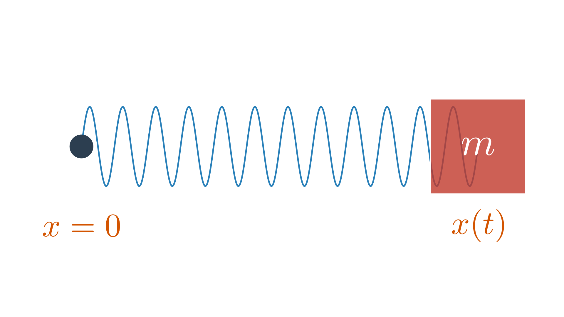
A one-dimensional mass–spring system.

In 1D, the kinetic energy is $T = \tfrac{1}{2} m \dot q^2$.

Hooke's Law. Force is linearly proportional to stretch in the spring: $\color{#ff7f0e}{f} = -k \, \color{#17becf}{x}$.

Since potential energy is the negative of mechanical work, \begin{equation} W = \int -k\, x(t)\, v(t)\, dt = \int -k\, x\, dx = -\tfrac{1}{2} k x^2 \;\implies\; V = \tfrac{1}{2} k q^2. \end{equation} Thus, \begin{equation} \begin{split} L &= \tfrac{1}{2} m \dot q^2 - \tfrac{1}{2} k q^2, \\\
\frac{d}{dt}\frac{\partial L}{\partial \dot q} &= \frac{d}{dt} (m \dot q), \\\
\frac{\partial L}{\partial q} &= -k q. \end{split} \end{equation} Using Euler–Lagrange: \begin{equation} m \ddot q = -k q. \end{equation}

Time Integration

Newton’s law, $m \ddot q = f(q)$, is a second-order ODE; it gives local information about curvature on a $t$ vs $q$ graph. Time integration generates the full function $q$ over time. Thus, generating an animation is equivalent to traversing this curve in time.

Input. An ODE, $\ddot q = f(q, \dot q)$ and initial conditions: $q_0 = \mathbf{q}(t_0)$, $\dot q_0 = \mathbf{\dot q}(t_0)$.

Output. A discrete update equation $\mathbf{q}^{t+1} = F(\mathbf{q}^t, \mathbf{q}^{t-1}, \ldots, \mathbf{\dot q}^t, \mathbf{\dot q}^{t-1}, \ldots)$.

Let us do this for the mass–spring system. We have a second-order ODE $m \ddot q = -k q$. Set $\dot q = v$ to get a first-order system $m \dot v = -k q$. In matrix form,

\[\begin{equation} \underbrace{\begin{pmatrix} m & 0 \\ 0 & 1 \end{pmatrix}}_{A} \underbrace{\frac{d}{dt} \begin{pmatrix} v \\ q \end{pmatrix}}_{\dot y} = \overbrace{\begin{pmatrix} 0 & -k \\ 1 & 0 \end{pmatrix} \underbrace{\begin{pmatrix} v \\ q \end{pmatrix}}_{y}}^{f(y)} \;\implies\; A \dot y = f(y). \end{equation}\]

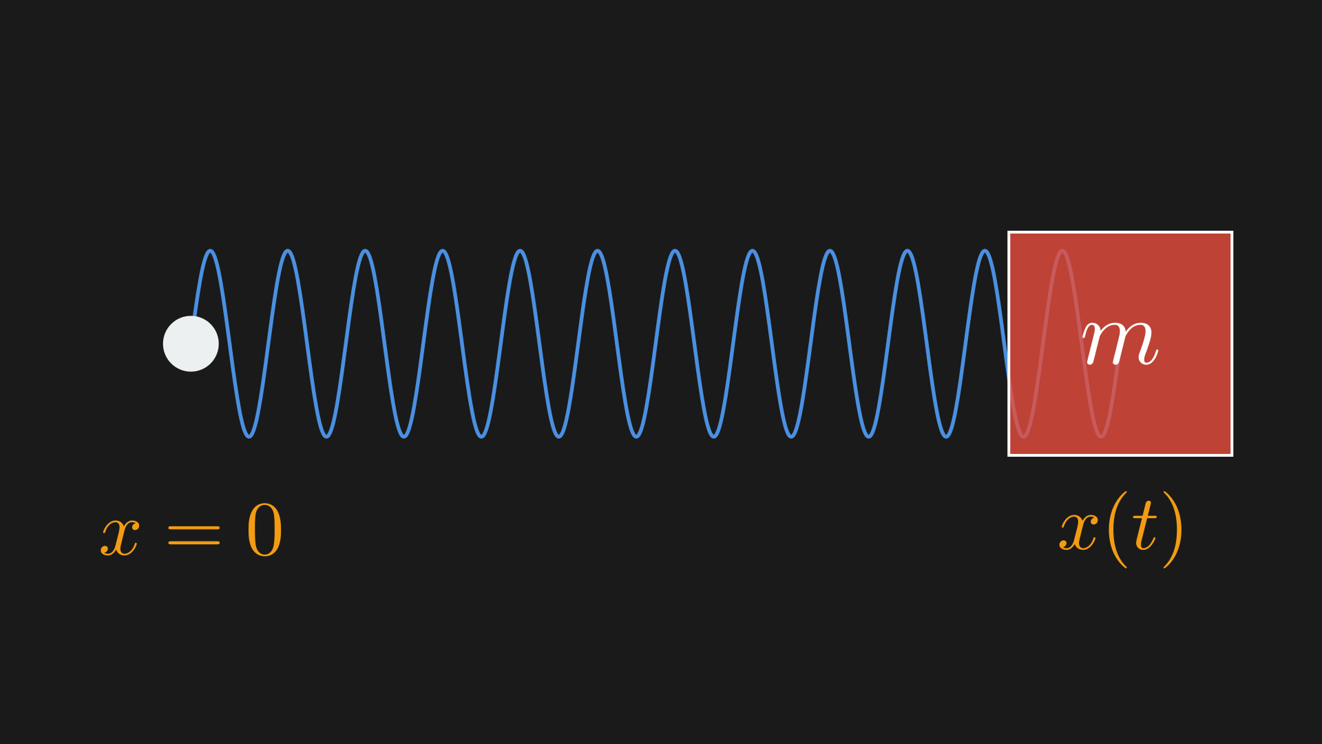
We can see that our ODE defines the vector field in the phase plane and the integration is a circle in this simple case.¹⁰

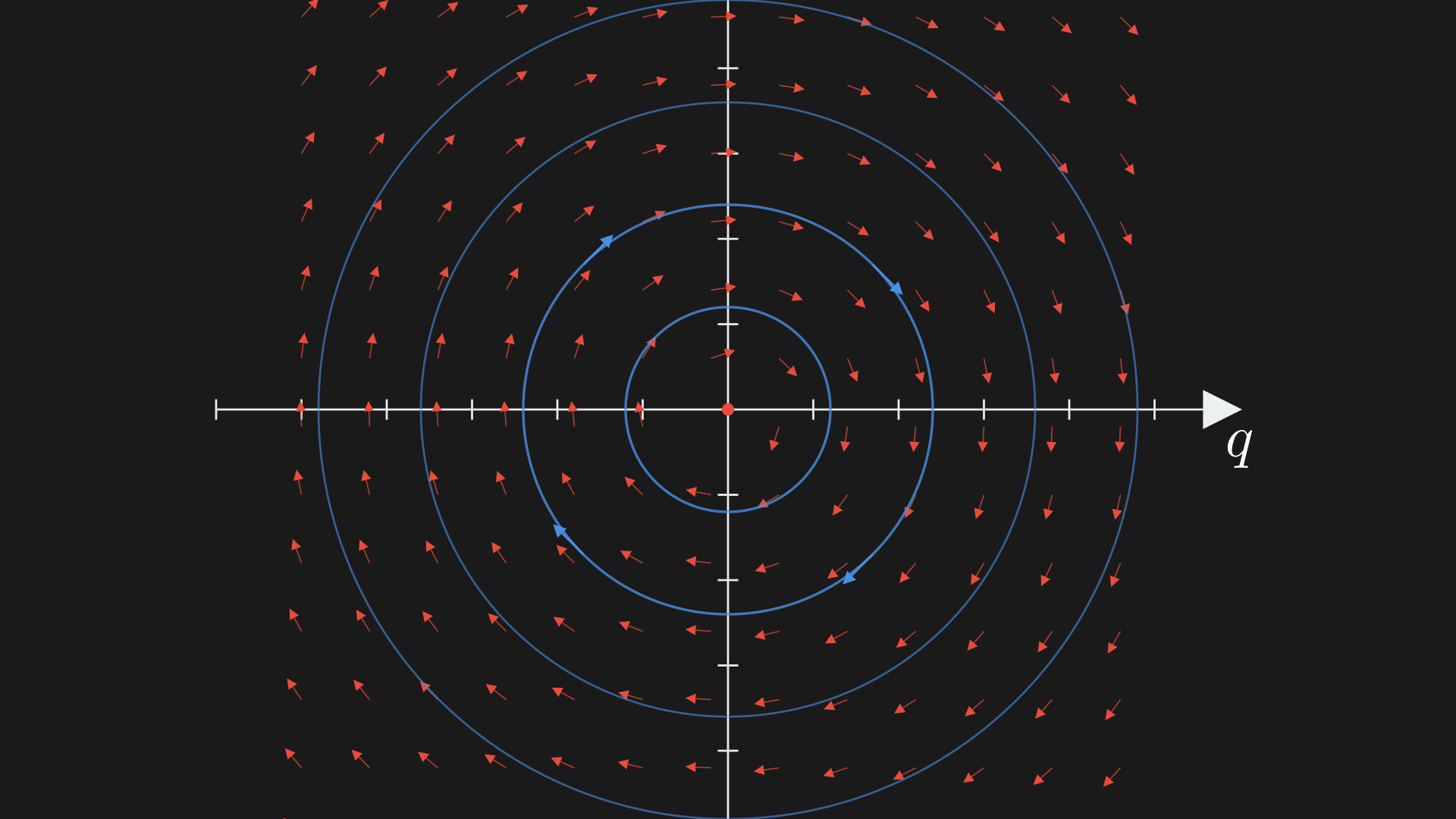Phase space for the linear spring–mass system. The vector field shows the flow $(\dot q,\dot v) = (v, -\tfrac{k}{m}\, q)$.

There are two types of time integration algorithms:

• explicit: the next time step uses only values at or before the current time
• implicit: the next time step uses values at the future time (solved implicitly)

Forward Euler Time Integration

Approximate the derivative with a first-order finite difference, \begin{equation} \dot y \approx \frac{1}{\Delta t} (y^{t+1}-y^t). \end{equation} Evaluate the function $f$ at the current timestep, \begin{equation} A \, \frac{1}{\Delta t} (y^{t+1}-y^t) = f(y^t) \;\implies\; y^{t+1} = y^t + \Delta t\, A^{-1} f(y^t). \end{equation} Now expand into individual update rules, \begin{equation} \begin{split} v^{t+1} &= v^t - \Delta t \, \frac{k}{m} q^t, \\
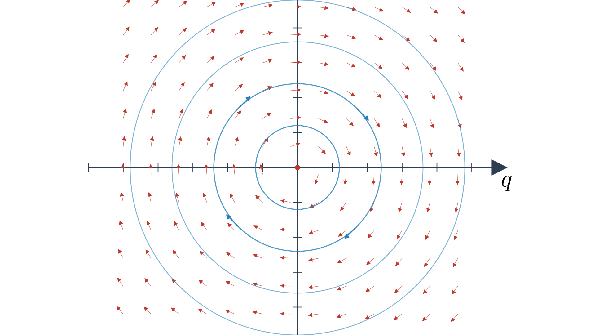
q^{t+1} &= q^t + \Delta t \, v^t. \end{split} \end{equation} Forward Euler is not numerically stable here; it spirals outwards (unbounded).¹¹

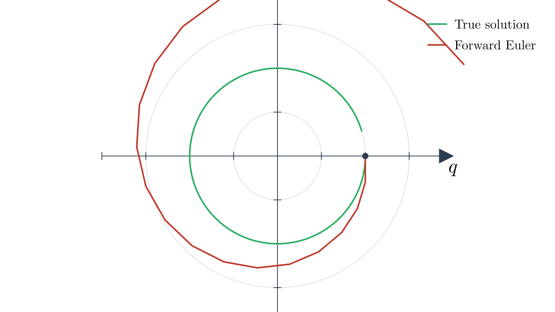
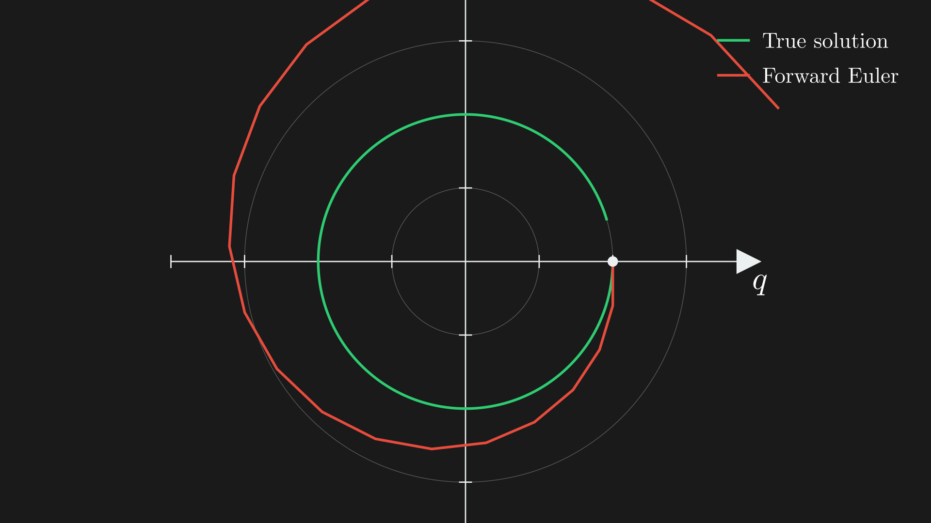Numerical instability of Forward Euler integration for the mass-spring system. The green curve shows the true circular trajectory that conserves energy, while the red spiral demonstrates how Forward Euler amplifies energy over time, causing the trajectory to grow unbounded despite starting from the same initial conditions.

Runge–Kutta Time Integration

Main idea: rather than using a single slope like Forward Euler, use multiple slopes.¹²

\(\begin{equation} y^{t+1} = y^t + \Delta t\\, A^{-1} \big( \alpha \\, \underbrace{f\big(y^{t+\overbrace{a}^{\text{time coefficient}}}\big)}_{\text{slope 1}} + \beta \\, \underbrace{f\big(\tilde y^{\\, t+\overbrace{b}^{\text{time coefficient}}}\big)}_{\text{slope 2}} \big). \end{equation}\) $y^{t+a}$ and $y^{t+b}$ are estimates at future timesteps obtained via Forward Euler, $\tilde y^{\, t+a} = y^t + a\, \Delta t\, A^{-1} f(y^t)$. $\alpha$ and $\beta$ are averaging coefficients.

A good choice is $a=0$, $b=1$, $\alpha=\beta=\tfrac{1}{2}$. With these we get Heun’s method, \begin{equation} y^{t+1} = y^t + \frac{\Delta t}{2} A^{-1}\big(f(y^t) + f(\tilde y^{\, t+1})\big), \qquad \tilde y^{\, t+1} = y^t + \Delta t \, A^{-1} f(y^t). \end{equation}

These can be written in a compact form as \begin{equation} \begin{split} \kappa_1 &= A^{-1} f(y^t), \\ \kappa_2 &= A^{-1} f\big(y^t + \Delta t \, \kappa_1\big), \\ y^{t+1} &= y^t + \frac{\Delta t}{2} (\kappa_1 + \kappa_2). \end{split} \end{equation}

One of the most popular approaches is fourth-order Runge–Kutta (RK4), which is quite stable, \begin{equation} \begin{split} \kappa_1 & = A^{-1} f\big(y^t\big), \\
\kappa_2 & = A^{-1} f\big(y^t+\tfrac{\Delta t}{2} \, \kappa_1\big), \\
\kappa_3 & = A^{-1} f\big(y^t+\tfrac{\Delta t}{2} \, \kappa_2\big), \\
\kappa_4 & = A^{-1} f\big(y^t+\Delta t \, \kappa_3\big), \\
\mathbf{y}^{t+1} &= \mathbf{y}^t + \frac{\Delta t}{6}\left(\kappa_1+2\kappa_2+2\kappa_3+\kappa_4\right). \end{split} \end{equation}

Backward Euler Time Integration

Start the same way as before, but evaluate the force at the next time step, \begin{equation} A \, \frac{1}{\Delta t}\left(y^{t+1}-y^t\right) = \underbrace{f\left(y^{t+1}\right)}_{\text{evaluated at next time step}}. \end{equation} However, unlike Runge–Kutta we do not use Forward Euler to get $y^{t+1}$; we truly do an implicit integration.

Let us make some notation to show that this is linear in $y$:

\[\begin{equation} \underbrace{\begin{pmatrix} m & 0 \\ 0 & 1 \end{pmatrix}}_{A} \underbrace{\frac{d}{dt} \begin{pmatrix} v \\ q \end{pmatrix}}_{\dot y} = \overbrace{\underbrace{\begin{pmatrix} 0 & -k \\ 1 & 0 \end{pmatrix}}_{B} \underbrace{\begin{pmatrix} v \\ q \end{pmatrix}}_{y}}^{f(y)} \;\implies\; A \dot y = B y. \end{equation}\]

Now write Backward Euler as

\[\begin{equation} A \, \frac{1}{\Delta t}\left(y^{t+1}-y^t\right) = \underbrace{B\, y^{t+1}}_{\text{evaluated at next time step}}. \end{equation}\]

Let us now write the update rule and simplify it,

\[\begin{equation} \begin{split} y^{t+1} &= y^t + \Delta t\, A^{-1} B\, y^{t+1}, \\ (\mathbb{I}-\Delta t\, A^{-1} B)\, y^{t+1} &= y^t. \end{split} \end{equation}\]

We can also write this in the following way, which will be useful for some analysis, \begin{equation} \underbrace{y^{t+1}-y^t}_{\text{vector between states}} = \overbrace{\Delta t\, A^{-1} B\, y^{t+1}}^{\text{slope at } t+1}. \end{equation} As in the phase portrait, Backward Euler slowly converges to the origin, where the block is at the wall with zero velocity and has lost all its energy. This damping is numerical, not physical; it makes the algorithm unconditionally stable, and can help model real-world damping effects.¹³

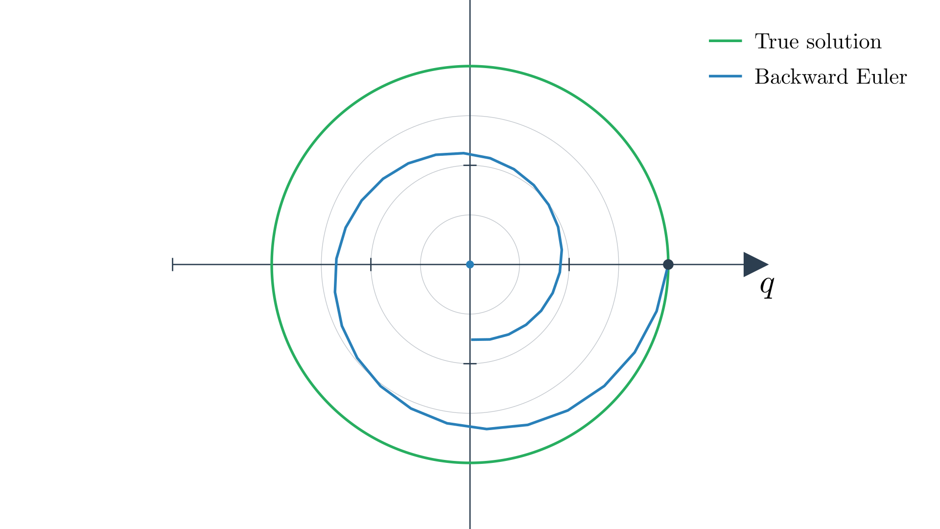
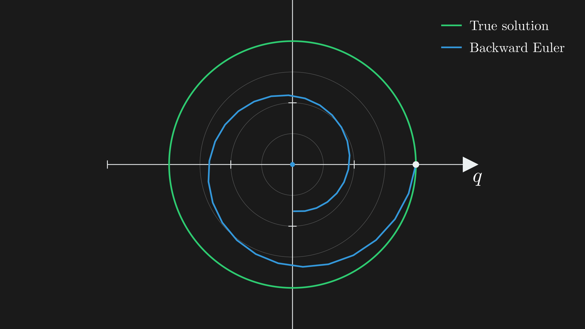Numerical damping in Backward Euler integration. The green curve shows the true energy-conserving circular trajectory, while the blue spiral demonstrates how Backward Euler introduces artificial damping, causing the trajectory to spiral inward toward the equilibrium point at the origin. This numerical dissipation makes the method unconditionally stable.

We can represent Backward Euler in terms of generalized position $q$ and velocity $v$, \begin{equation} \begin{split} & (\mathbb{I}-\Delta t\, A^{-1} B)\, y^{t+1}=y^t, \\\
& v^{t+1}+\Delta t\, \frac{k}{m} \, q^{t+1}=v^t \quad\quad q^{t+1}-\Delta t\, v^{t+1}=q^t, \\\
& v^{t+1}+\Delta t\, \frac{k}{m}\left(q^t+\Delta t\, v^{t+1}\right)=v^t \;\text{ (by plugging in $q^{t+1}-\Delta t\, v^{t+1}=q^t$)}, \\\
& \left(1+\Delta t^2 \, \frac{k}{m}\right) v^{t+1}=v^t-\Delta t \, \frac{k}{m} \, q^t \quad\quad q^{t+1}=q^t+\Delta t\, v^{t+1}. \end{split} \end{equation}

Symplectic Euler Time Integration

• First take an explicit velocity step \begin{equation} v^{t+1}=v^t-\Delta t \, \frac{k}{m} \, q^t. \end{equation}
• Next take an implicit position step \begin{equation} q^{t+1}=q^t+\Delta t \, v^{t+1}. \end{equation} If we do this just right, we can cancel the exploding and damping. A property is that our simulation can survive until infinity if we do this.

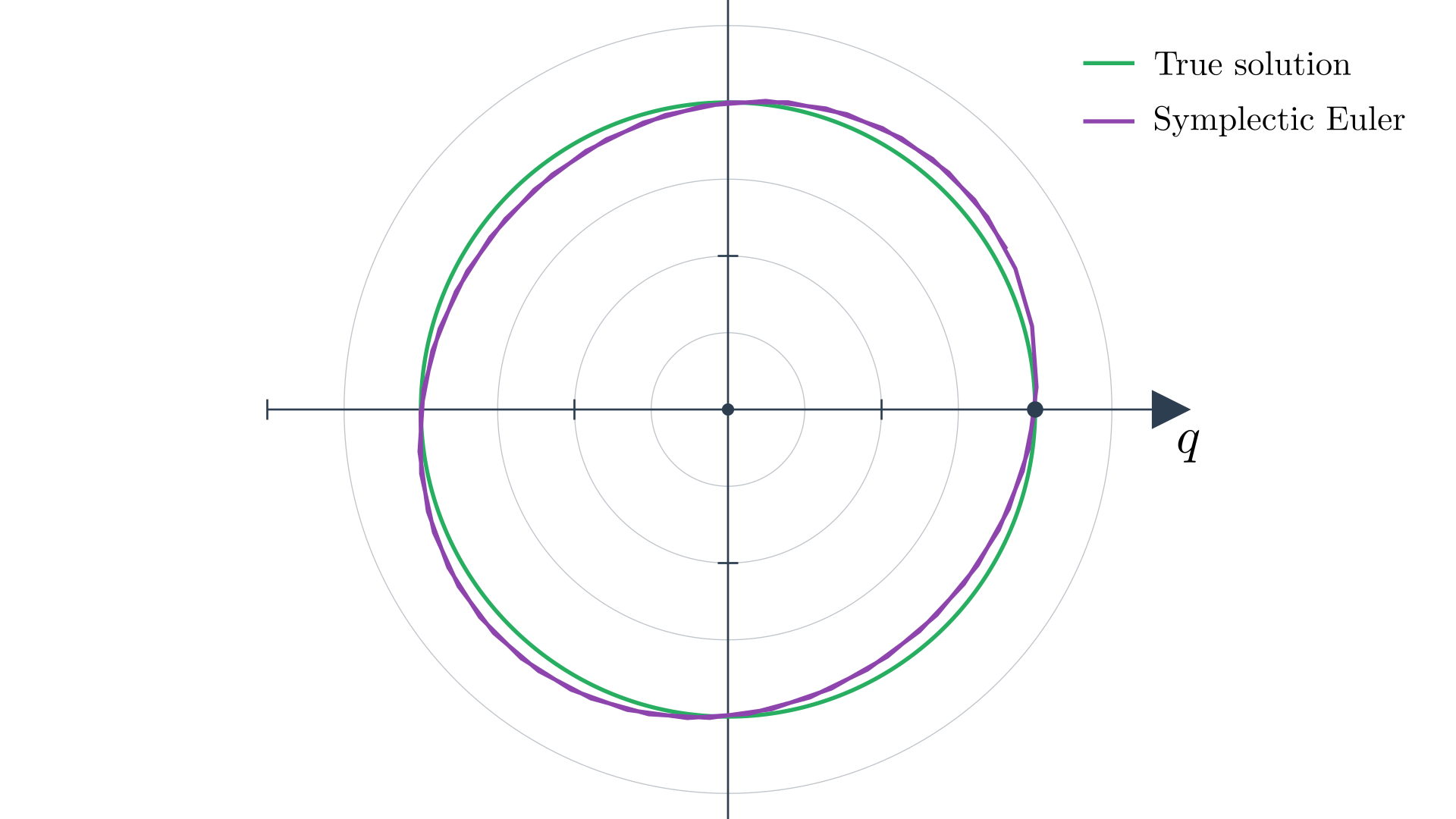
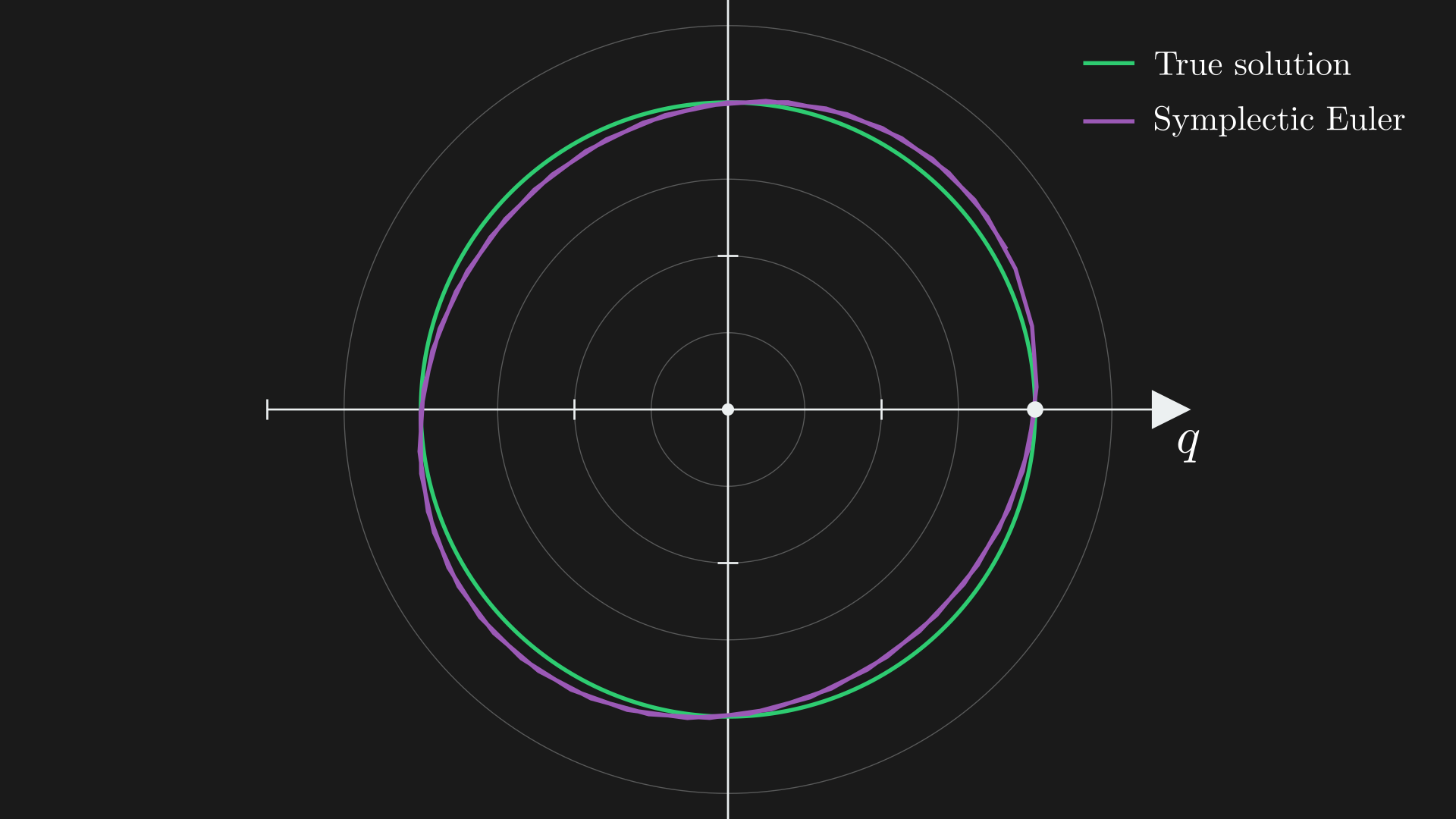Symplectic Euler integration preserves system structure. The green curve shows the true energy-conserving circular trajectory, while the purple trajectory demonstrates how Symplectic Euler maintains bounded, stable motion over long time periods. Unlike Forward Euler (unstable) or Backward Euler (damped), this method preserves the symplectic structure of systems.

Mass–Spring Systems in 3D

We can first get generalized coordinates and generalized velocity of the spring–mass system. Suppose there are two particles at positions $\color{#17becf}{x_0}$ and $\color{#17becf}{x_1}$ at the two ends of the spring, \begin{equation} \dot q = \begin{pmatrix} \dot x_0 \\\ \dot x_1 \end{pmatrix} = \begin{pmatrix} v_0 \\\ v_1 \end{pmatrix}. \end{equation} Thus the kinetic energy is $\tfrac{1}{2} m \lVert v_0 \rVert_2^2$ and so on. The total kinetic energy is \begin{equation} \color{#2ca02c}{T} = \sum_{i=0}^1 \frac{1}{2} m \, v_i^\top v_i = \sum_{i=0}^1 \frac{1}{2} v_i^\top \begin{pmatrix} m & 0 & 0\\\ 0 & m & 0\\\ 0 & 0 & m \end{pmatrix} v_i = \frac{1}{2} \dot q^\top \color{#2c3e50}{M} \, \dot q, \end{equation} where $\color{#2c3e50}{M}$ is the block diagonal mass matrix with two $3\times 3$ particle mass matrices on the diagonal, so $M \in \mathbb{R}^{6\times 6}$.

For potential energy we want:

• the spring should return to its rest length when all external forces are removed
• rigid motions should not change energy
• energy should depend only on particle positions

We first define the strain, \(\underbrace{\color{#17becf}{\ell}}_{\color{#17becf}{\text{deformed length}}}-\overbrace{\color{#008080}{\ell_0}}^{\color{#008080}{\text{rest length}}}\). However, $\ell=\ell_0$ is not a global minimum, so define potential energy as $\tfrac{1}{2}k(\ell-\ell_0)^2$, where $k$ is a stiffness parameter. To define the length we have \begin{equation} \Delta x = x_1-x_0 = \underbrace{\begin{pmatrix} -\mathbb{I} \; & \; \mathbb{I} \end{pmatrix}}_{B} \overbrace{\begin{pmatrix} x_0 \\\\ x_1 \end{pmatrix}}^{q} \;\implies\; \ell = \sqrt{\Delta x^\top \Delta x} = \sqrt{q^\top B^\top B q}. \end{equation} Thus, the Lagrangian looks like \begin{equation} L = \frac{1}{2} \dot q^\top M \, \dot q - \frac{1}{2} k\left(\sqrt{q^\top B^\top B q} - \color{#008080}{\ell_0}\right)^2. \end{equation} Our Euler–Lagrange equation simplifies since only $V$ depends on $q$: \begin{equation} \frac{d}{dt}\frac{\partial L}{\partial \dot q} = -\frac{\partial V}{\partial q} \;\triangleq\; f(q). \end{equation} We can simplify the left-hand side as \begin{equation} \begin{split} \frac{d}{dt}\frac{\partial L}{\partial \dot q} &= \frac{d}{dt}\frac{\partial}{\partial \dot q}\left(\frac{1}{2}\, \dot q^\top M \, \dot q\right) \\\
&= \frac{d}{dt}\, (M\, \dot q) \\\
&= M \, \ddot q \quad \text{(since $M$ is constant)} \\\
\implies\quad \color{#2c3e50}{M}\, \color{#d62728}{\ddot q} &= -\frac{\partial V}{\partial q}. \end{split} \end{equation}

Representing Meshes

To represent a mesh we can think of each vertex as a mass and each edge as a spring. The block diagonal mass for the entire mesh is \begin{equation} \color{#2c3e50}{M} = \begin{pmatrix} M_0 & \cdots & 0 \\\
\vdots & \ddots & \vdots \\\
0 & \cdots & M_{n-1} \end{pmatrix} \in \mathbb{R}^{3n \times 3n}. \end{equation} We can compute kinetic and potential energies by summing over all individual energies. Define $q_j$ as

\[\begin{equation} q_j = \begin{pmatrix} x_a \\ x_b \end{pmatrix} = \underbrace{\overbrace{\begin{pmatrix} X_1 \\ x_b \end{pmatrix}}^{\color{#8c564b}{\text{selection matrix}}}}_{\color{#8c564b}{E_j}} \, q. \end{equation}\]

Here, $\color{#8c564b}{E_j}$ is a binary selection (gather) matrix that extracts the two endpoints of spring $j$ from the global vector $q$.¹⁴

So our Lagrangian for a mesh looks like \begin{equation} L = \frac{1}{2}\, \dot q^\top M \, \dot q - \sum_{j=0}^{m-1} V_j(E_j q). \end{equation} We can compute the generalized forces as

\[\begin{equation} \begin{split} -\frac{\partial V}{\partial q} &= -\frac{\partial}{\partial q} \sum_{j=0}^{m-1} V_j(E_j q) \\ &= - \sum_{j=0}^{m-1} E_j^T \frac{\partial V_j}{\partial q_j}(q_j) \;\underbrace{(q_j)}_{\text{per-spring gradient}} \\ &= \sum_{j=0}^{m-1} E_j^T f_j(q_j) \;\underbrace{(q_j)}_{\text{per-spring generalized force}}. \end{split} \end{equation}\]

Linearly-Implicit Time Integration

We will start with Backward Euler:

\(\begin{equation} \begin{split} M\dot{q}^{\, t+1} &= M\dot{q}^{\, t} + \Delta t\, f(q^{t+1}) \quad\; \text{(Backward Euler)}, \\ q^{t+1} &= q^t + \Delta t\, \dot{q}^{\, t+1}, \\ M\dot{q}^{\, t+1} &= M\dot{q}^{\, t} + \Delta t\, f(\underbrace{q^t + \Delta t\, \dot{q}^{\, t+1}}_{\text{Substitute}}), \\ M\dot{q}^{\, t+1} &\approx M\dot{q}^{\, t} + \Delta t\, f(q^t) + \underbrace{\Delta t^2 \, \frac{\partial f}{\partial q}\, \dot{q}^{\, t+1}}_{\text{stiffness matrix }\, \color{#c0392b}{K}} \quad \text{(first order)}, \\ (M - \Delta t^2 K)\, \dot{q}^{\, t+1} &= M\dot{q}^{\, t} + \Delta t\, f(q^t) \quad \text{(solve linear system)}, \\ q^{t+1} &= q^t + \Delta t\, \dot{q}^{\, t+1} \quad \text{(update position)}. \end{split} \end{equation}\) This is a first-order linearization of the force map around $q^t$.¹⁵

We still need to figure out the stiffness matrix $\color{#c0392b}{K}$,¹⁶ \begin{equation} \begin{split} K &= \frac{\partial f}{\partial q} \quad \text{(by definition)},\\\
\; f &= -\frac{\partial}{\partial q} \sum_{j=0}^{m-1} V_j(E_j q),\\\
\color{#c0392b}{K} &= -\frac{\partial^2}{\partial q^2} \sum_{j=0}^{m-1} V_j(E_j q)\\\
&= -\sum_{j=0}^{m-1} \frac{\partial^2}{\partial q^2} V_j(E_j q)\\\
&= \sum_{j=0}^{m-1} \left(-E_j^T \frac{\partial^2 V_j}{\partial q_j^2} E_j\right)\\\
&= \sum_{j=0}^{m-1} \left(E_j^T \color{#c0392b}{K_j} E_j\right). \end{split} \end{equation} So $K$ is the negative Hessian (matrix of second derivatives) of the potential energy. A per-spring stiffness matrix is \begin{equation} \color{#c0392b}{K_j} = -\frac{\partial^2 V_j}{\partial q_j^2}. \end{equation} The individual stiffness matrix is $12\times 12$ and is assembled as in the figure.

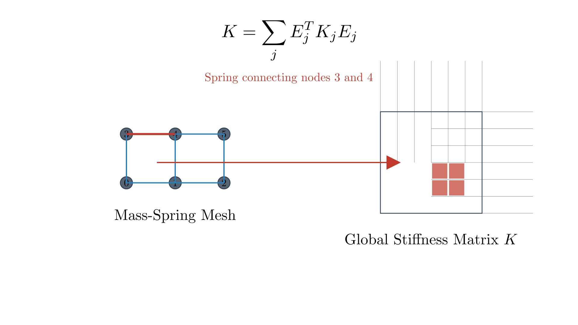
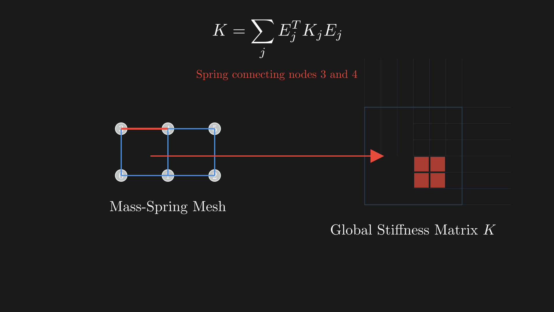Assembly of the global stiffness matrix from per-spring contributions. The mesh on the left shows numbered nodes connected by springs. Each spring contributes a local stiffness matrix $K_j$ that is assembled into the global matrix $K$ using selection matrices: $K = \sum_j E_j^T K_j E_j$. The highlighted spring and corresponding matrix entries demonstrate how individual springs create sparse contributions to specific matrix locations.

How to Add Constraints

We may want invisible constraints like fixing the position of certain vertices (red dots in our demo) so they can never move. To enforce $q_i = b_i$, define a reduced set of DOFs¹⁷

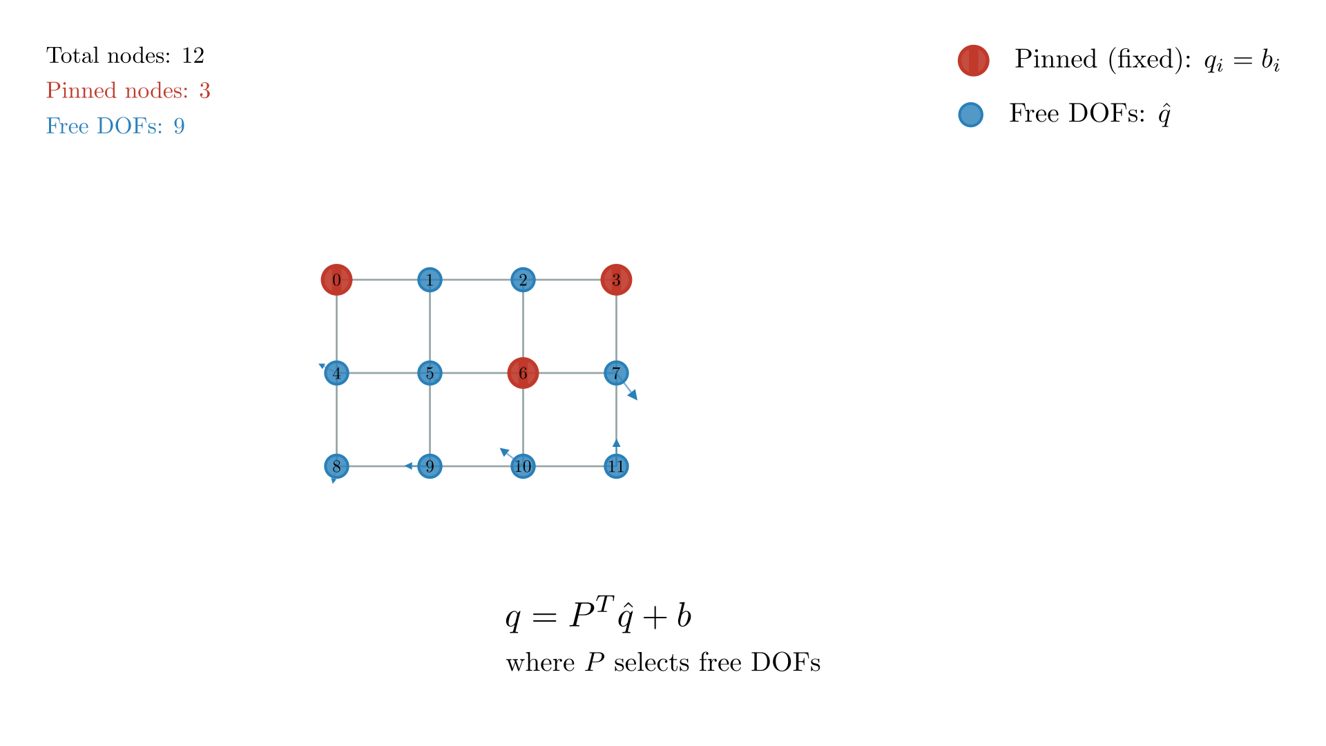
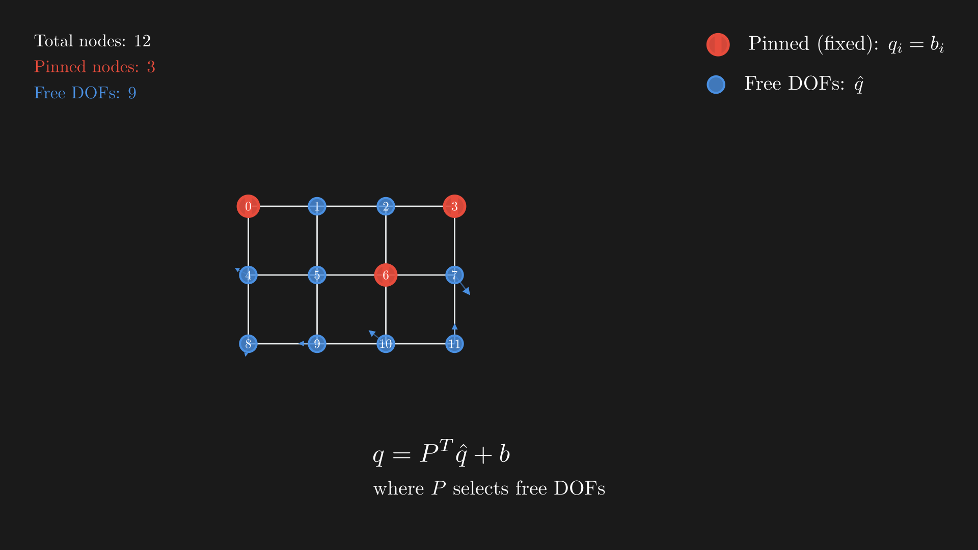Constraint enforcement in mass-spring systems. Red nodes with pins are fixed (pinned) constraints where $q_i = b_i$, while blue nodes represent free degrees of freedom $\hat{q}$. Small arrows on free nodes indicate possible displacements. The constraint reduction $q = P^T\hat{q} + b$ transforms the system from 12 total DOFs to 9 free DOFs by eliminating the 3 pinned nodes.

\[\begin{equation} \underbrace{\hat{q}}_{\text{DOF}} = \overbrace{\color{#2c3e50}{P}}^{\color{#2c3e50}{\text{select non-fixed points}}}\\, q. \end{equation}\]

Then \begin{equation} P^T\hat{q} = \overbrace{\begin{pmatrix} x_0 \\
x_1 \\
x_2 \\
0 \\
\vdots \\
x_n \end{pmatrix} + \underbrace{\begin{pmatrix} 0 \\
0 \\
0 \\
\color{#e67e22}{b_i} \\
\vdots \\
0 \end{pmatrix}}_{\color{#e67e22}{b}}}^{q}. \end{equation} Thus, with $q=P^T\hat{q} + \color{#e67e22}{b}$ and $\dot q = P^T \dot{\hat{q}}$ we get \begin{equation} \begin{split} P\left(M - \Delta t^2 K\right)P^T\, \dot{\hat{q}}^{\, t+1} &= P M\, \dot{q}^{\, t} + \Delta t\, P f(q^t), \\\
q^{t+1} &= q^t + \Delta t\, P^T \dot{\hat{q}}^{\, t+1}. \end{split} \end{equation}

Citation

Please cite this work as:

Rishit Dagli. "Hopefully the Most Gentle Introduction to Simulation". Rishit Dagli's Blog (September 2025). https://rishit-dagli.github.io/2025/09/27/simulation.html

Or use the BibTex citation:

@article{ dagli2025hopefully, title = { Hopefully the Most Gentle Introduction to Simulation }, author = { Rishit Dagli }, journal = {rishit-dagli.github.io}, year = { 2025 }, month = { September }, url = "https://rishit-dagli.github.io/2025/09/27/simulation.html" }