.png)

As children squabble, they will often start naming large numbers to win arguments. Sometimes it’s “times a million” or “times a bajillion” but once a kid learns about infinity, it eventually ends with “times infinity”. What do you do when you are on the receiving end of infinity? You can half-heartedly attempt a “times infinity + 1” but you know infinity is as big as it gets. Nothing can be bigger than that…right?
Well, it turns out that not all infinities are equal, some are larger than others! And in some ways, you can actually do “infinity + 1”.
Comparing Finite Collections
What does it mean for one infinity to be larger than another infinity?
Let’s start by thinking about what it means for one integer to be larger than another integer. When we say n>mn > m, for example, we are saying that a collection of nn objects would be bigger than a collection of mm objects.
But what does it mean for the collection to be “bigger”? If the size of the collection is more fundamental than numbers, then how can we compare sizes without numbers?
Well, we know that the bigger collection is big enough to “contain” the smaller collection. So we could pair off objects from both collections, till one collection runs out of items. When that happens, the collection with items left over is the bigger collection!
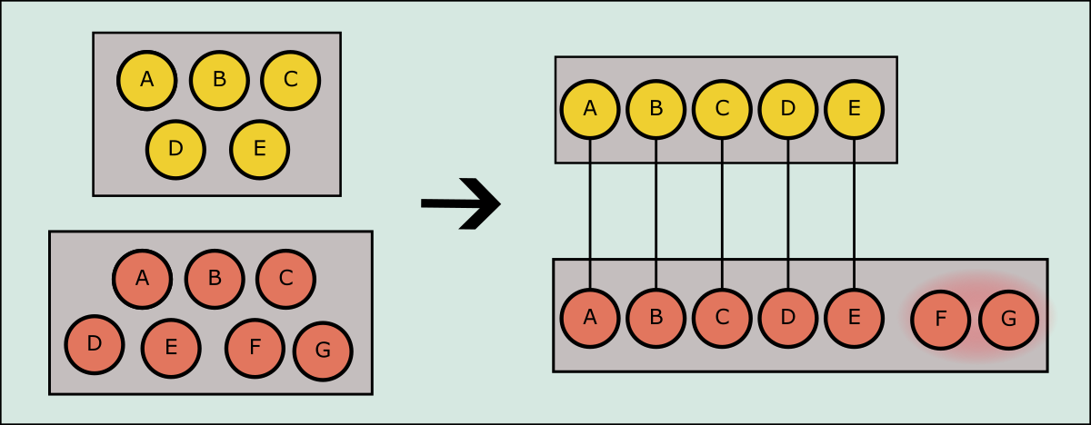
Two sets can be compared by pairing off items. Since all the items in the top set can be paired off but not all the items in the bottom set could be paired off, we know that the bottom set is bigger.
We can carry over the same logic when comparing infinite sets. If there is a pairing strategy such that all items from set NN can be paired off with items from set MM, but the reverse can’t be done then set NN is smaller than set MM.
Integer Subsets
Let’s try out our system on some infinite sets. Let OO be the set of all odd numbers and let EE be the set of all even numbers.
O={1,3,5,…} E={2,4,6…} O = \lbrace 1, 3, 5, … \rbrace \\\ E = \lbrace 2, 4, 6… \rbrace
Are there more odd numbers or even numbers? Well, for any odd number, we can pair it to a unique even number by adding one to it.
f(o)=o+1 f(o) = o + 1
We can similarly, pair every even number to a unique odd number by subtracting one from it.
g(e)=e−1 g(e) = e - 1
Since both pairings cover all elements in both directions, the sets must be equal in size. This tells us that there are as many odd numbers as even!
Let’s get a little crazier. What about the set of all perfect squares? How does it compare to all the positive integers?
N={1,2,3,4,…} S={1,4,9,16,…} \begin{aligned} N &= \lbrace 1, 2, 3, 4, … \rbrace \\\ S &= \lbrace 1, 4, 9, 16, … \rbrace \end{aligned}
There are obviously many integers missing in the set of perfect squares. Can they be the same size despite the “holes”? Let’s see if we can find a mapping between them. By definition, each perfect square can be mapped to a unique integer (using the square root). Each integer can also be mapped to a unique perfect square by just squaring the number. So with these mappings, we can exhaustively pair off all the items.
f(s)=s g(n)=n2 \begin{aligned} f(s) &= \sqrt{s} \\\ g(n) &= n^2 \end{aligned}
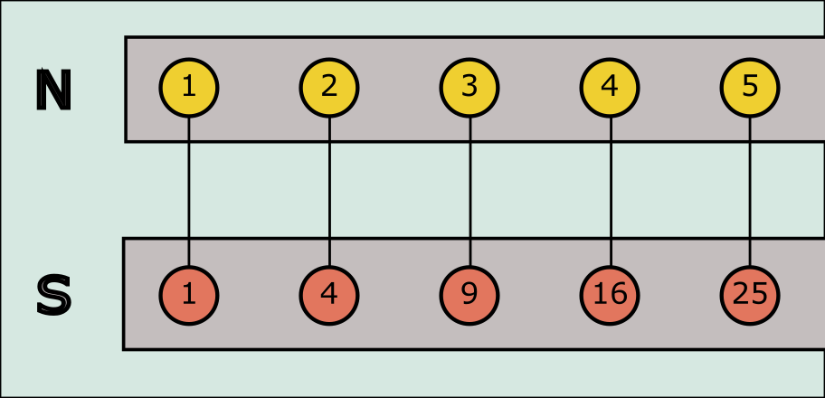
While the set of perfect squares skips many numbers, it can still be paired off with the set of integers.
So the set of perfect squares and the set of all integers are the same size! It doesn’t matter that the set of perfect squares has “holes” compared to set of all the integers. They are the same size because you can map the sets to each other.
Number Classes
Okay, this is cool but I seem to be making the opposite argument. I keep showing infinite sets that are the same size! Where are the infinite sets with different sizes?
Let’s start by recalling some classification of numbers:
- N\mathbb N is the set of positive integers. Examples: 1,2,31, 2, 3
- Z\mathbb Z is the set of all integers. Examples: −1,0,1-1, 0, 1
- Q\mathbb Q, the rationals, is the set of all numbers that can be expressed as a ratio of two integers. Examples: 12,31,54\frac 1 2, \frac 3 1, \frac 5 4
- R\mathbb R, the reals, are the set of all numbers (rationals and irrationals). Examples: π,e,2\pi, e, \sqrt 2
The positive integers (N\mathbb N) are also called the counting numbers because we use those numbers to count. Really, when we map a set to the positive integers, we are actually just “counting” the members of that set. For example, when we mapped the integers to the perfect squares (1→11 \rightarrow 1, 2→42 \rightarrow 4), it really is the same as us counting the perfect squares! 1 is the first perfect square, 4 is the second perfect square and so on.
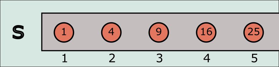
Perfect squares can be counted. Note, that the pattern is basically the same as when we “mapped” the perfect squares to the positive integers.
This is why the size of the positive integers (N\mathbb N) is called countable infinity. Anything that can be counted, can be mapped to the positive integers and therefore has the same size as N\mathbb N.
For a set to be countable, the counting order doesn’t have to be straightforward like the order for the perfect squares. The order can be anything arbitrary as long as we can show that it covers all the elements of the set. For example, the set of all integers (Z\mathbb Z) is also countably infinite. We can show this by “counting” all the integers in this alternating order:
Animation of counting all the integers. You can do this by alternating between the positive and negative numbers such that you cover all the integers one by one! [code]
By alternating between the positive and the negative integers, we can count all the integers. This essentially maps all the integers to the positive integers, showing that the sets have the same size: countable infinity.
Rationals (Q\mathbb Q)
Similarly, the rational numbers can be counted as well. To count them, we just have to come up with a listing order that will guarantee that we don’t miss any rational numbers in the list.
One strategy to do this is to list rational numbers with small numerators and denominators first and go “up” from there. More specifically, we can order all rational numbers by the sum of the numerator and the denominator.
So we start with all fractions that add up to 2, which is just 11\frac 1 1. Then we list all fractions that add up to 3, which are 21,12\frac 2 1, \frac 1 2. Then we list all fractions that add up to 4: 13,22,31\frac 1 3, \frac 2 2, \frac 3 1. We can keep going up from there. Since we go through all possible sums, we will enumerate all possible fractions. Some fractions are double counted, like 22\frac 2 2 which is the same as 11\frac 1 1, but we can easily skip them when we are counting them.
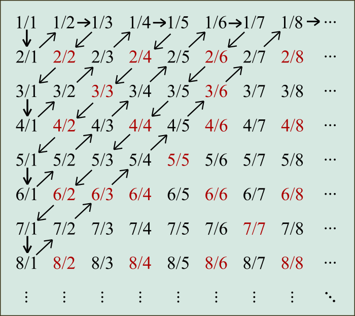
Rational numbers can be counted by ordering them by the sum of the numerator and denominator and then by skipping over non-reduced fractions (shown in red). Source: wikipedia.
With this listing strategy we can “count” all the rational numbers which means the rational numbers are countably infinite.
Reals (R\mathbb R)
So there is countable infinity, and anything that can be counted has the same size as countable infinity. So something to be bigger than countable infinity, that something has to be uncountable. But can’t everything be counted?
Turns out the answer is no! Georg Cantor proved that the real numbers cannot be counted. The trick Cantor used is famously called Cantor’s diagonal argument. Let’s walk through the argument.
To begin, let’s assume that the real numbers are countable. So, there is some order we can count the numbers in such that we won’t miss any numbers. Let’s write the numbers down in that order. For convenience, let’s write down the numbers in binary using 0’s and 1’s.
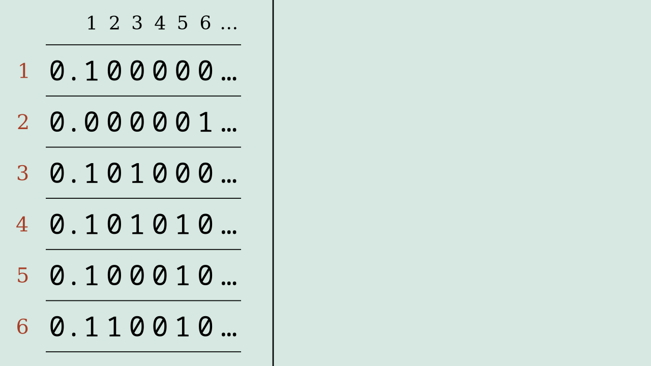
A hypothetical list that lists all real numbers between 0 and 1. Each row is a number with potentially infinite digits. We only show 6 numbers but this list keeps going to infinity.
This hypothetical list is supposed to include all possible real numbers. If we can find a number that is missing in the list, then we can show that the list is incomplete. If we can make this strategy generic and apply to all possible lists, then we have shown that a complete list of all real numbers is impossible.
One such strategy is to craft a number that is guaranteed to be missing. We can build this number to be different from every number in this list. We can do this by iterating through the numbers in the list and iterating through their digits.
For the first digit, we can pick the first number (0.100000…0.100000…) and look at its first digit (11). If we make our number have the opposite value (00), then we guarantee that our number will be different from the first number. Similarly, for the second digit, we can pick the second number (0.000001…0.000001…) and look at its second digit (00). If we make our number have the opposite value (11), then we guarantee that our number will be different from the second number. And then we can continue this process for every digit, making sure that we are different from each number in the list.
Visualization of Cantor’s diagonal argument. We construct a new number by going through the list one by one. For each row, we pick the next digit and make our constructed number have the opposite value. This guarantees that our constructed number differs from every number in at least one digit. [code]
Our strategy is generic and will apply to any counted list of real numbers. Given any list, we can always find a real number that’s missing. This means a complete list could never be built and therefore the real numbers cannot be counted. The set of real numbers is larger than the set of integers. That’s why the size of the real numbers is called uncountable infinity.
Continuum Hypothesis
So, the set of real numbers are bigger than the set of integers, but how much bigger? Can we relate the two infinities to make more sense of it?
Power Sets
Before we take that journey, let’s take a quick detour and learn about power sets.
A set contains items. A power set contains all the different sets you can make with the items from the original set.
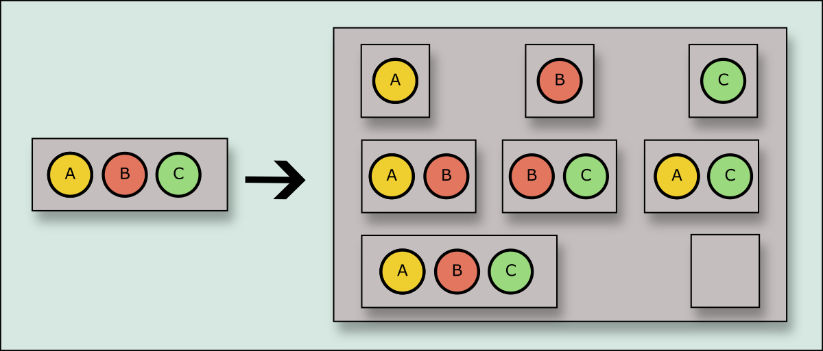
If a set is a box of objects, then the power set is the box of boxes. The power set contains boxes with all possible combinations of the objects.
So a power set represents all the different combinations you can make. The power set operation is so common that it even has a standard symbol P(s)\mathcal P(s).
Since the power set contains all the different combinations, the size of the power set grows exponentially. In our example, the size of the set (∣s∣|s|) was 33 and the size of the power set (∣P(s)∣|\mathcal P(s)|) was 88 (which is 232^3).
More generally, the size of the power set can be described in terms of the size of the original set as:
∣P(s)∣=2∣s∣ |\mathcal P(s)| = 2^{|s|}
Comparing Infinities
The reason we talked about power set is that the real numbers can be thought of as the power set of the integers.
To see how, we start by noting that real numbers have infinite digits. But the digits are countably infinite because we can just count the digits in order.
So each real number is “countably” long.
This becomes even cleaner if we write the real number in binary notation. Each digit will have a value between {0,1}\lbrace 0, 1 \rbrace. Then we can note down all the digits that are set to 11. Since any digit that is not set to 1, is set to 0, we can uniquely identify this number by just noting down which digits have the value of 1.
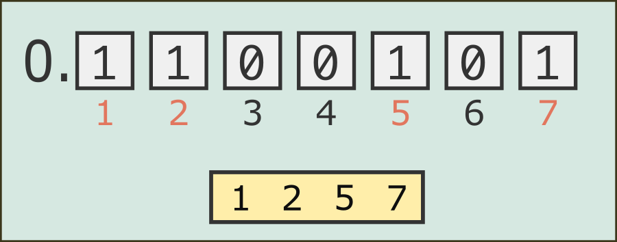
A real number can be uniquely mapped to a subset of integers by noting down all digits that equal to 1 in binary notation.
When we write the digits down though, we have written down a set of integers that uniquely represents the real number. In our example, 0.11001010.1100101 uniquely maps to {1,2,5,7}\{1, 2, 5, 7\}.
Since the process we described would work for any number, every real number maps to a set of integers.
So, one real number maps to a set of all integers. The set of all real numbers maps to the set of all possible sets of integers. We just learned that the “set of all possible sets of S” is the power set of S.
So, the set of real numbers maps to the power set of the integers.
R=P(N) \mathbb R = \mathcal P(\mathbb N)
What about the sizes of these sets?
Countable infinity, which is the size of the natural numbers, is also referred to as ℵ0\aleph_0 (“aleph nought”). Uncountable infinity, the size of the real numbers, is referred to as c\mathfrak c (for “continuum”). And since the size of a power set is 2x2^x where xx is the size of the set, we can also relate the sizes of the infinite sets as:
∣R∣=∣P(N)∣ c=2ℵ0 \begin{aligned} |\mathbb R| &= |\mathcal P(\mathbb N)|\\\ \mathfrak c &= 2^{\aleph_0} \end{aligned}
So we have found a cool relationship between the two sizes of infinity. Uncountable infinity is as big as the power set of countable infinity!
Now the interesting question is: is there an infinity that has a size in between these two infinities (ℵ0\aleph_0, 2ℵ02^{\aleph_0}).
If we let ℵn\aleph_n represent the n-th smallest infinity, we can rephrase this to ask if ℵ1=2ℵ0\aleph_1 = 2^{\aleph_0} (which says “is the next largerst infinity the same as the power set of the integers”). The Continuum Hypothesis (CH) claims that there is no intermediate infinity and thus the above statement is true.
In the same way that the real numbers can be generated by taking the power set of the integers, we can generate an even larger infinity by taking the power set of the real numbers. And then we can keep generating bigger infinities by taking their power sets.
This leads to a more general question: is there an infinity with a size between an infinite set and its power set? Which is the same as asking whether this is true for all α\alpha:
ℵα+1=2ℵα \aleph_{\alpha+1} = 2^{\aleph_\alpha}
If this is true, then all possible infinities can be generated by starting with the integers and repeatedly taking the power set of the generated set. The hypothesis that this is true is called the General Continuum Hypothesis (GCH).
So according to the GCH, we indeed can do “infinity + 1” by taking the power set and finding the next larger infinity!
ZFC and Logical Independence
But is the General Continuum Hypothesis true? To answer this question, we have to decide what it even means for something to be true.
Mathematical statements are true when they are proven by other true statements. And those true statements are usually proven from other proven statements, recursively leading to a set of axioms that are assumed to be true and self-evident.
There are many ways to axiomatize different fields of mathematics. For over a century, though, the game plan has been to axiomatize a fundamental theory about sets and then use that theory to prove the rest of mathematics. This plan fell into a bit of a crisis when paradoxes like Russell’s paradox were discovered, but eventually a set of axioms was defined that felt natural and avoided those paradoxes. This set of axioms is called ZFC (Zermelo-Fraenkel + Axiom of Choice, which is a nonsensical acronym).
So, ZFC is the foundation of all of modern mathematics. And that can help us decide what it means for something to be true in this context. When we say something is true, we are implying that the statement is provable by the axioms of ZFC.
Great, so is GCH provable by the axioms of ZFC? No. So is it provable that GCH is false? Also, no!
It turns out that ZFC is logically independent of the General Continuum Hypothesis!
Just like you can use numbers to count different types of objects or use geometry to describe physical buildings or computer graphics, ZFC can be used to work with different “models” of sets. GCH is true in some models and false in others.
Matter of fact, there is another weird thing that is logically independent of ZFC: the existence of an Inaccessible Cardinal (which sounds more like a bird than the inaccessible rail).
We established that you can keep getting a bigger infinity (ℵκ+1\aleph_{\kappa + 1}) by taking the power set of the previous infinite set. Now imagine repeating this operation infinite times. Imagine doing it countably infinite times. Then imagine doing it uncountably many times. Then imagine doing it (ℵκ\aleph_{\kappa}) times for any κ\kappa that you can imagine. These are all “accessible” because they can be reached.
An inaccessible cardinal is an infinity that is so big that this repeating process will never reach that size of infinity. It is literally inaccessible. Does such an infinite size exist? It may or may not exist depending on the model and/or additional assumptions that you choose.
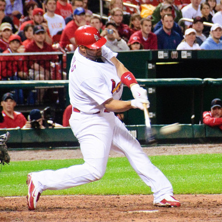
Albert Pujols, a large Cardinal whose existence is also independent of ZFC. image
There is actually a host of “large cardinals” that may or may not exist depending on your choice of model/assumptions. The large cardinals also have fun names to capture their ridiculousness: ethereal, ineffable, remarkable, superstrong, huge, superhuge.
So the next time you get in a numerical repartee with a 10-year-old, make sure you establish which model of ZFC you are working in first.


![Cute, but powerful: meet NanoCluster, a tiny supercomputer [video]](https://www.youtube.com/img/desktop/supported_browsers/chrome.png)
