.png)

How do we actually evaluate LLMs?
It’s a simple question, but one that tends to open up a much bigger discussion.
When advising or collaborating on projects, one of the things I get asked most often is how to choose between different models and how to make sense of the evaluation results out there. (And, of course, how to measure progress when fine-tuning or developing our own.)
Since this comes up so often, I thought it might be helpful to share a short overview of the main evaluation methods people use to compare LLMs. Of course, LLM evaluation is a very big topic that can’t be exhaustively covered in a single resource, but I think that having a clear mental map of these main approaches makes it much easier to interpret benchmarks, leaderboards, and papers.
I originally planned to include these evaluation techniques in my upcoming book, Build a Reasoning Model (From Scratch), but they ended up being a bit outside the main scope. (The book itself focuses more on verifier-based evaluation.) So I figured that sharing this as a longer article with from-scratch code examples would be nice.
In Build A Reasoning Model (From Scratch), I am taking a hands-on approach to building a reasoning LLM from scratch.
If you liked “Build A Large Language Model (From Scratch)”, this book is written in a similar style in terms of building everything from scratch in pure PyTorch.
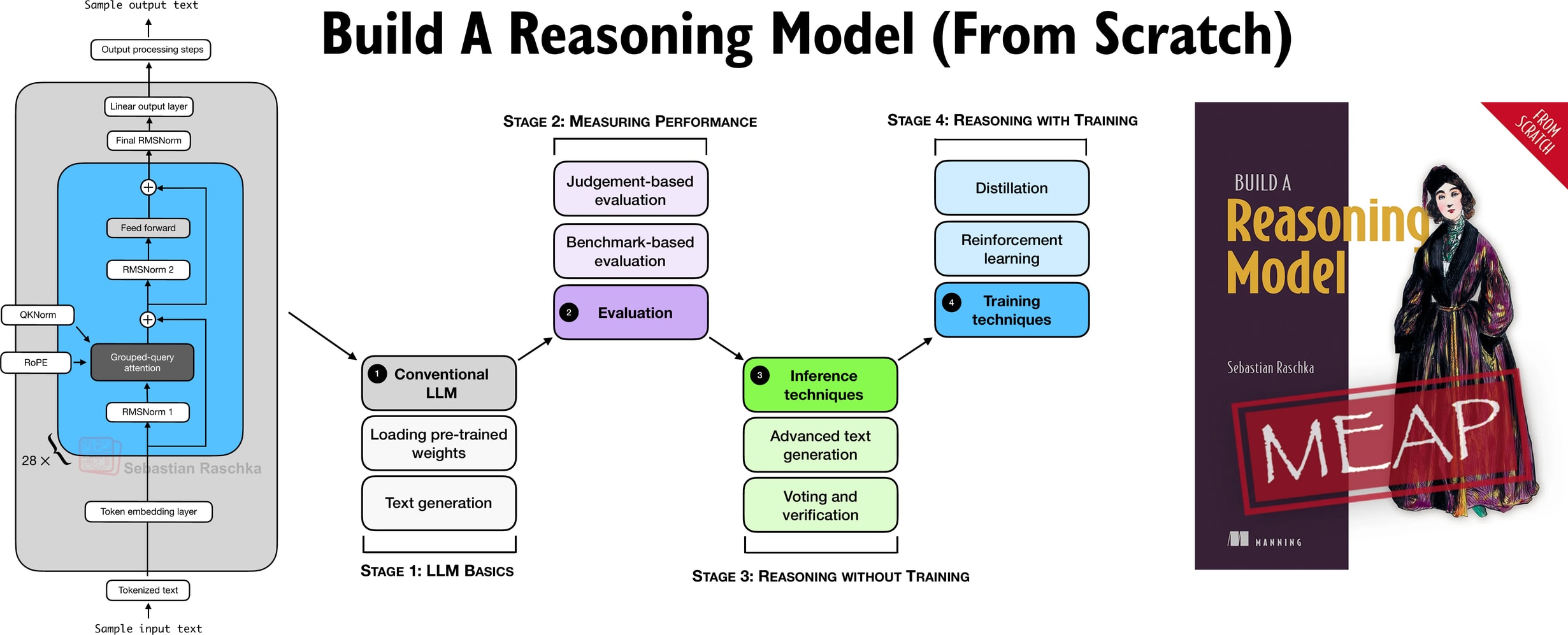
The book is currently in early-access with >100 pages already online, and I have just finished another 30 pages that are currently being added by the layout team. If you joined the early access program (a big thank you for your support!), you should receive an email when those go live.
PS: There’s a lot happening on the LLM research front right now. I’m still catching up on my growing list of bookmarked papers and plan to highlight some of the most interesting ones in the next article.
But now, let’s discuss the four main LLM evaluation methods along with their from-scratch code implementations to better understand their advantages and weaknesses.
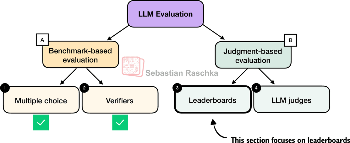
There are four common ways of evaluating trained LLMs in practice: multiple choice, verifiers, leaderboards, and LLM judges, as shown in Figure 1 below. Research papers, marketing materials, technical reports, and model cards (a term for LLM-specific technical reports) often include results from two or more of these categories.
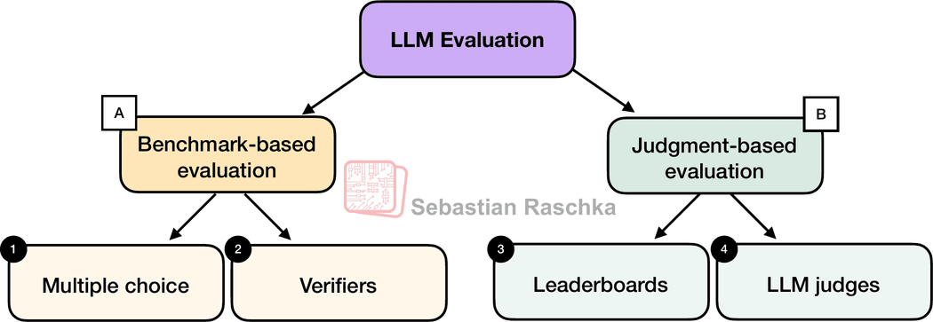
Furthermore the four categories introduced here fall into two groups: benchmark-based evaluation and judgment-based evaluation, as shown in the figure above.
(There are also other measures, such as training loss, perplexity, and rewards, but they are usually used internally during model development.)
The following subsections provide brief overviews and examples of each of the four methods.
We begin with a benchmark‑based method: multiple‑choice question answering.
Historically, one of the most widely used evaluation methods is multiple-choice benchmarks such as MMLU (short for Massive Multitask Language Understanding, https://huggingface.co/datasets/cais/mmlu). To illustrate this approach, figure 2 shows a representative task from the MMLU dataset.
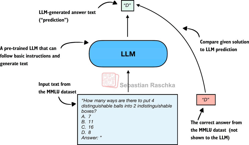
Figure 2 shows just a single example from the MMLU dataset. The complete MMLU dataset consists of 57 subjects (from high school math to biology) with about 16 thousand multiple-choice questions in total, and performance is measured in terms of accuracy (the fraction of correctly answered questions), for example 87.5% if 14,000 out of 16,000 questions are answered correctly.
Multiple-choice benchmarks, such as MMLU, test an LLM’s knowledge recall in a straightforward, quantifiable way similar to standardized tests, many school exams, or theoretical driving tests.
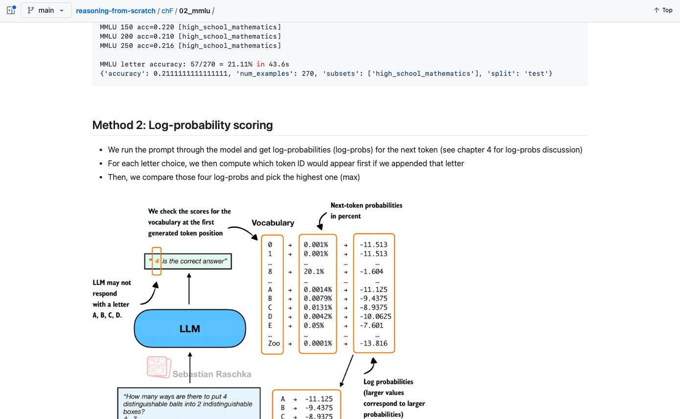
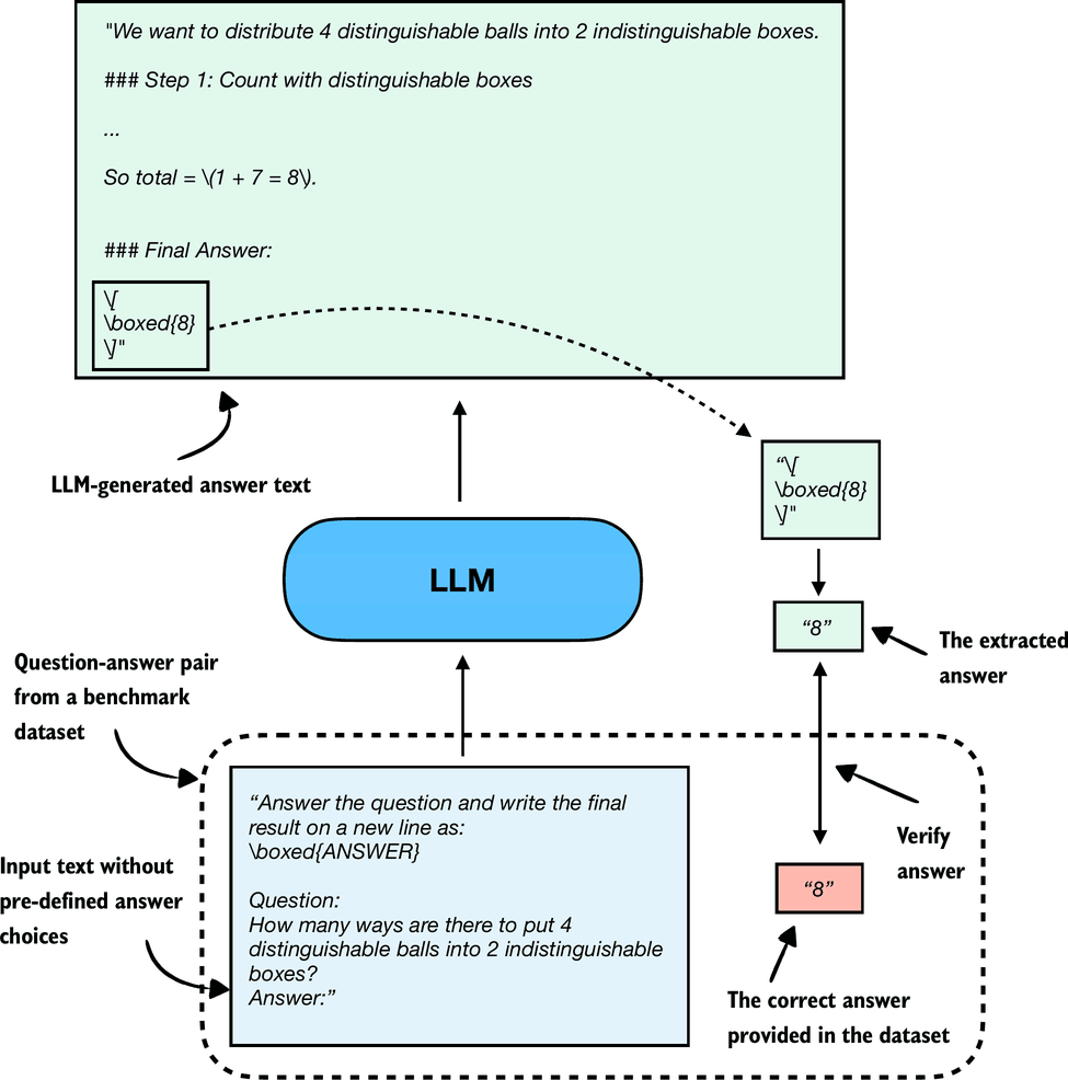
Note that figure 2 shows a simplified version of multiple-choice evaluation, where the model’s predicted answer letter is compared directly to the correct one. Two other popular methods exist that involve log-probability scoring. I implemented them here on GitHub. (As this builds on the concepts explained here, I recommended checking this out after completing this article.)
The following subsections illustrate how the MMLU scoring shown in figure 2 can be implemented in code.
First, before we can evaluate it on MMLU, we have to load the pre-trained model. Here, we are going to use a from-scratch implementation of Qwen3 0.6B in pure PyTorch, which requires only about 1.5 GB of RAM.
Note that the Qwen3 model implementation details are not important here; we simply treat it as an LLM we want to evaluate. However, if you are curious, a from-scratch implementation walkthrough can be found in my previous Understanding and Implementing Qwen3 From Scratch article, and the source code is also available here on GitHub.
Instead of copy & pasting the many lines of Qwen3 source code, we import it from my reasoning_from_scratch Python library, which can be installed via
pip install reasoning_from_scratchor
uv add reasoning_from_scratchfrom pathlib import Path import torch from reasoning_from_scratch.ch02 import get_device from reasoning_from_scratch.qwen3 import ( download_qwen3_small, Qwen3Tokenizer, Qwen3Model, QWEN_CONFIG_06_B ) device = get_device() # Set matmul precision to "high" to # enable Tensor Cores on compatible GPUs torch.set_float32_matmul_precision("high") # Uncomment the following line # if you encounter device compatibility issues # device = "cpu" # Use the base model by default WHICH_MODEL = "base" if WHICH_MODEL == "base": download_qwen3_small( kind="base", tokenizer_only=False, out_dir="qwen3" ) tokenizer_path = Path("qwen3") / "tokenizer-base.json" model_path = Path("qwen3") / "qwen3-0.6B-base.pth" tokenizer = Qwen3Tokenizer(tokenizer_file_path=tokenizer_path) elif WHICH_MODEL == "reasoning": download_qwen3_small( kind="reasoning", tokenizer_only=False, out_dir="qwen3" ) tokenizer_path = Path("qwen3") / "tokenizer-reasoning.json" model_path = Path("qwen3") / "qwen3-0.6B-reasoning.pth" tokenizer = Qwen3Tokenizer( tokenizer_file_path=tokenizer_path, apply_chat_template=True, add_generation_prompt=True, add_thinking=True, ) else: raise ValueError(f"Invalid choice: WHICH_MODEL={WHICH_MODEL}") model = Qwen3Model(QWEN_CONFIG_06_B) model.load_state_dict(torch.load(model_path)) model.to(device) # Optionally enable model compilation for potential performance gains USE_COMPILE = False if USE_COMPILE: torch._dynamo.config.allow_unspec_int_on_nn_module = True model = torch.compile(model)In this section, we implement the simplest and perhaps most intuitive MMLU scoring method, which relies on checking whether a generated multiple-choice answer letter matches the correct answer. This is similar to what was illustrated earlier in Figure 2, which is shown below again for convenience.
For this, we will work with an example from the MMLU dataset:
example = { "question": ( "How many ways are there to put 4 distinguishable" " balls into 2 indistinguishable boxes?" ), “choices”: ["7", "11", "16", "8"], “answer”: "D", }Next, we define a function to format the LLM prompts.
def format_prompt(example): return ( f"{example['question']}\n" f"A. {example['choices'][0]}\n" f"B. {example['choices'][1]}\n" f"C. {example['choices'][2]}\n" f"D. {example['choices'][3]}\n" "Answer: " ) # Trailing space in "Answer: " encourages a single-letter next tokenLet’s execute the function on the MMLU example to get an idea of what the formatted LLM input looks like:
prompt = format_prompt(example) print(prompt)The output is:
How many ways are there to put 4 distinguishable balls into 2
indistinguishable boxes?
The model prompt, as shown above, provides the model with a list of the different answer choices and ends with an “Answer: “ text that encourages the model to generate the correct answer.
While it is not strictly necessary, it can sometimes also be helpful to provide additional questions along with the correct answers as input, so that the model can observe how it is expected to solve the task. (For example, cases where 5 examples are provided are also known as 5-shot MMLU.) However, for current generations of LLMs, where even the base models are quite capable, this is not required.
Loading different MMLU samples
You can load examples from the MMLU dataset directly via the datasets library (which can be installed via pip install datasets or uv add datasets):
from datasets import load_dataset configs = get_dataset_config_names("cais/mmlu") dataset = load_dataset("cais/mmlu", "high_school_mathematics") # Inspect the first example from the test set: example = dataset["test"][0] print(example)Above, we used the “high_school_mathematics” subset; to get a list of the other subsets, use the following code:
from datasets import get_dataset_config_names subsets = get_dataset_config_names(”cais/mmlu”) print(subsets)Next, we tokenize the prompt and wrap it in a PyTorch tensor object as input to the LLM:
prompt_ids = tokenizer.encode(prompt) prompt_fmt = torch.tensor(prompt_ids, device=device) # Add batch dimension: prompt_fmt = prompt_fmt.unsqueeze(0)Then, with all that setup out of the way, we define the main scoring function below, which generates a few tokens (here, 8 tokens by default) and extracts the first instance of letter A/B/C/D that the model prints.
from reasoning_from_scratch.ch02_ex import ( generate_text_basic_stream_cache ) def predict_choice( model, tokenizer, prompt_fmt, max_new_tokens=8 ): pred = None for t in generate_text_basic_stream_cache( model=model, token_ids=prompt_fmt, max_new_tokens=max_new_tokens, eos_token_id=tokenizer.eos_token_id, ): answer = tokenizer.decode(t.squeeze(0).tolist()) for letter in answer: letter = letter.upper() # stop as soon as a letter appears if letter in "ABCD": pred = letter break if pred: break return predWe can then check the generated letter using the function from the code block above as follows:
pred1 = predict_choice(model, tokenizer, prompt_fmt) print( f"Generated letter: {pred1}\n" f"Correct? {pred1 == example['answer']}" )The result is:
Generated letter: C Correct? FalseAs we can see, the generated answer is incorrect (False) in this case.
This was just one of the 270 examples from the high_school_mathematics subset in MMLU. The screenshot (Figure 4) below show’s the performance of the base model and reasoning variant when executed on the complete subset. The code for this is available here on GitHub.
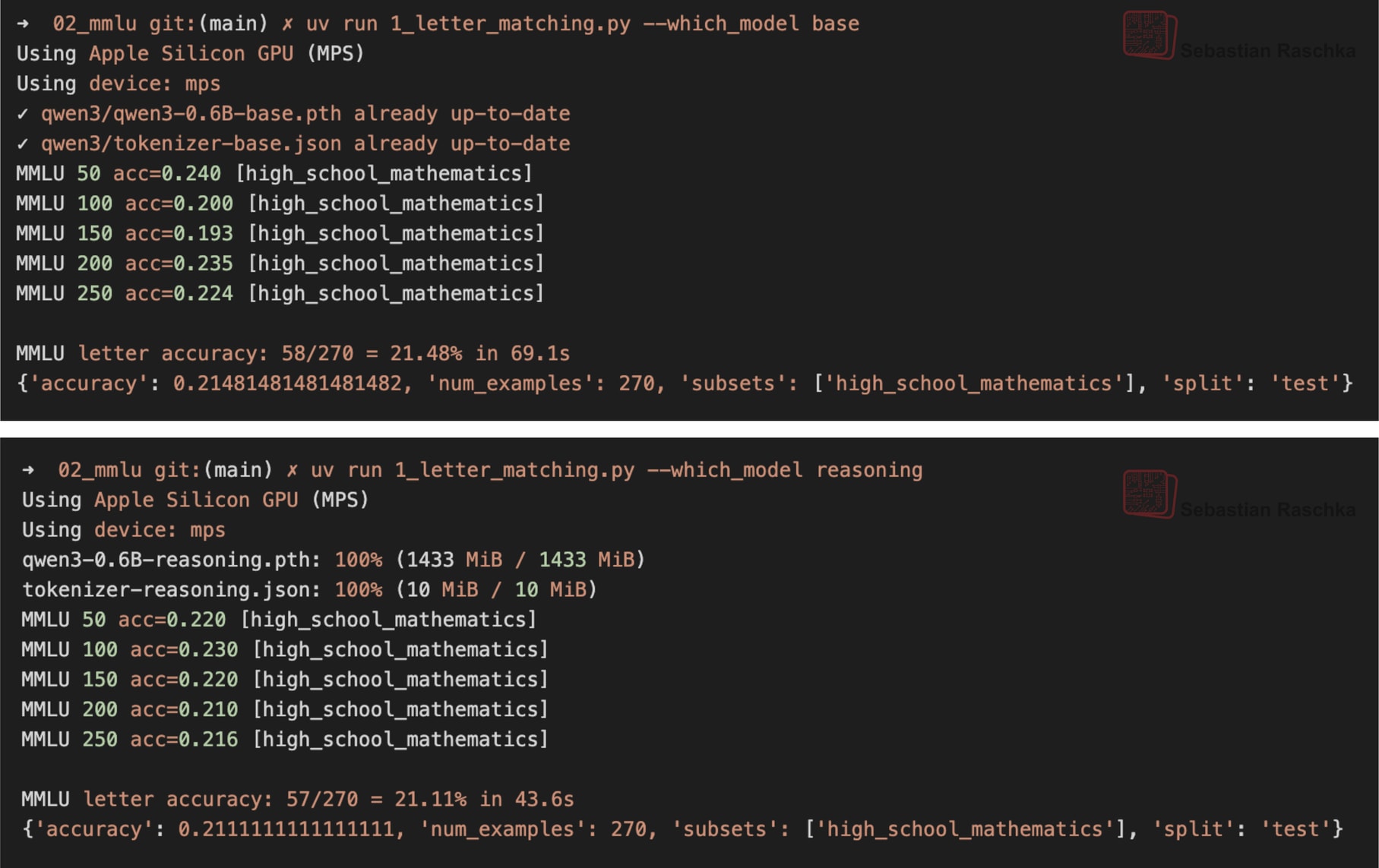
Assuming the questions have an equal answer probability, a random guesser (with uniform probability choosing A, B, C, or D) is expected to achieve 25% probability. So the both the base and reasoning model are not very good.
Multiple-choice answer formats
Note that this section implemented a simplified version of multiple-choice evaluation for illustration purposes, where the model’s predicted answer letter is compared directly to the correct one. In practice, more widely used variations exist, such as log-probability scoring, where we measure how likely the model considers each candidate answer rather than just checking the final letter choice. (We discuss probability-based scoring in chapter 4.) For reasoning models, evaluation can also involve assessing the likelihood of generating the correct answer when it is provided as input.
However, regardless of which MMLU scoring variant we use, the evaluation still amounts to checking whether the model selects from the predefined answer options.
A limitation of multiple‑choice benchmarks like MMLU is that they only measure an LLM’s ability to select from predefined options and thus is not very useful for evaluating reasoning capabilities besides checking if and how much knowledge the model has forgotten compared to the base model. It does not capture free-form writing ability or real-world utility.
Still, multiple-choice benchmarks remain simple and useful diagnostics: for example, a high MMLU score doesn’t necessarily mean the model is strong in practical use, but a low score can highlight potential knowledge gaps.
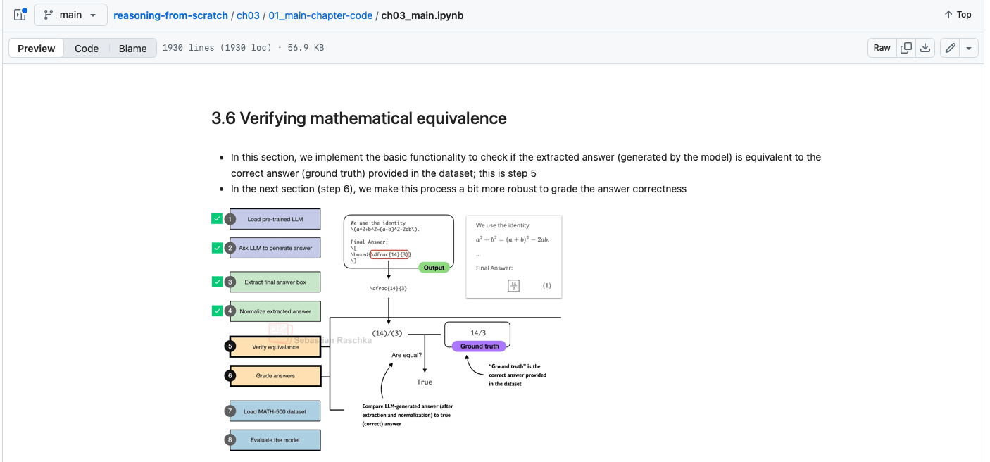
Related to multiple-choice question answering discussed in the previous section, verification-based approaches quantify the LLMs capabilities via an accuracy metric. However, in contrast to multiple-choice benchmarks, verification methods allow LLMs to provide a free-form answer. We then extract the relevant answer portion and use a so-called verifier to compare the answer portion to the correct answer provided in the dataset, as illustrated in Figure 6 below.
When we compare the extracted answer with the provided answer, as shown in figure above, we can employ external tools, such as code interpreters or calculator-like tools/software.
The downside is that this method can only be applied to domains that can be easily (and ideally deterministically) verified, such as math and code. Also, this approach can introduce additional complexity and dependencies, and it may shift part of the evaluation burden from the model itself to the external tool.
However, because it allows us to generate an unlimited number of math problem variations programmatically and benefits from step-by-step reasoning, it has become a cornerstone of reasoning model evaluation and development.
I wrote a comprehensive 35-page on this topic in my “Build a Reasoning Model (From Scratch)” book, so I am skipping the code implementation here. (I submitted the chapter last week. If you have the early access version, you’ll receive an email when it goes live and will be able to read it then. In the meantime, you can find the step-by-step code here on GitHub.)
So far, we have covered two methods that offer easily quantifiable metrics such as model accuracy. However, none of the aforementioned methods evaluate LLMs in a more holistic way, including judging the style of the responses. In this section, as illustrated in Figure 8 below, we discuss a judgment-based method, namely, LLM leaderboards.
The leaderboard method described here is a judgment-based approach where models are ranked not by accuracy values or other fixed benchmark scores but by user (or other LLM) preferences on their outputs.
A popular leaderboard is LM Arena (formerly Chatbot Arena), where users compare responses from two user-selected or anonymous models and vote for the one they prefer, as shown in Figure 9.
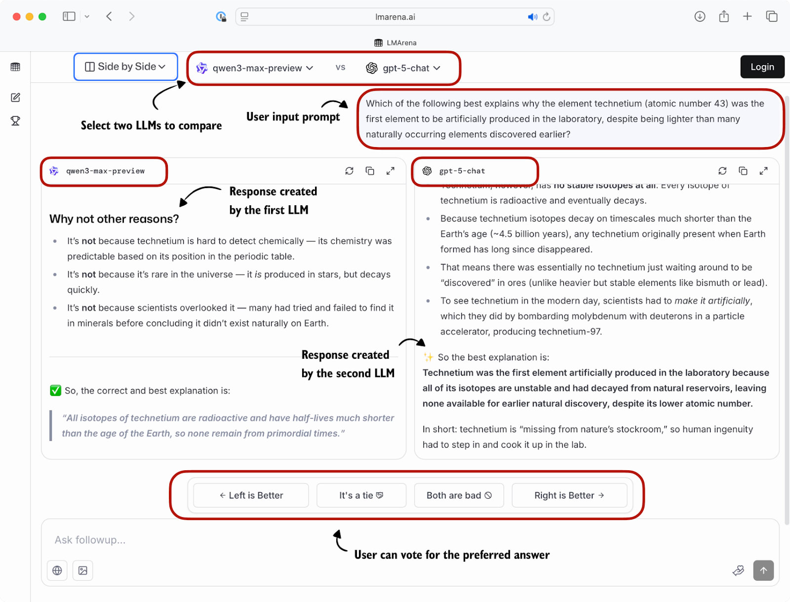
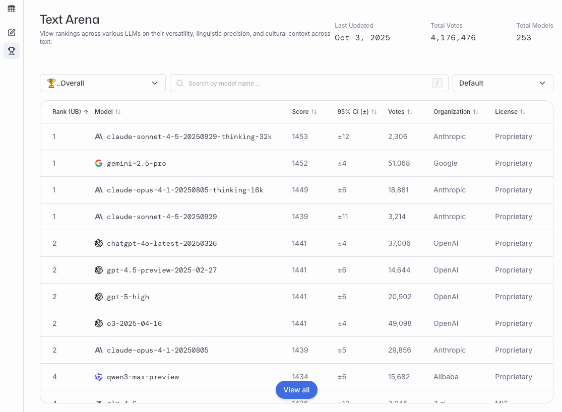
These preference votes, which are collected as shown in the figure above, are then aggregated across all users into a leaderboard that ranks different models by user preference. A current snapshot of the LM Arena leaderboard (accessed on October 3, 2025) is shown below in Figure 10.
In the remainder of this section, we will implement a simple example of a leaderboard.
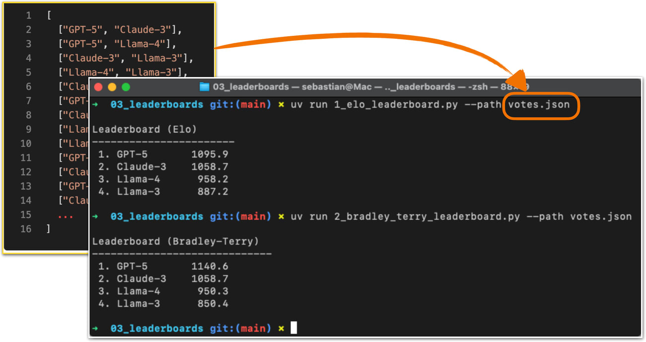
To create a concrete example, consider users prompting different LLMs in a setup similar to Figure 9. The list below represents pairwise votes where the first model is the winner:
votes = [ ("GPT-5", "Claude-3"), ("GPT-5", "Llama-4"), ("Claude-3", "Llama-3"), ("Llama-4", "Llama-3"), ("Claude-3", "Llama-3"), ("GPT-5", "Llama-3"), ]In the list above, each tuple in the votes list represents a pairwise preference between two models, written as (winner, loser). So, (“GPT-5”, “Claude-3”) means that a user preferred GPT-5 over a Claude-3 model answer.
In the remainder of this section, we will turn the votes list into a leaderboard. For this, we will use the popular Elo rating system, which was originally developed for ranking chess players.
Before we look at the concrete code implementation, in short, it works as follows. Each model starts with a baseline score. Then, after each comparison and the preference vote, the model’s rating is updated. Specifically, if a user prefers a current model over a highly ranked model, the current model will get a relatively large ranking update and rank higher in the leaderboard. Vice versa, if the current model loses against a lowly ranked model, it increases the rating only a little. (And if the current model loses, it is updated in a similar fashion, but with ranking points getting subtracted instead of added.)
The code to turn these pairwise rankings into a leaderboard is shown in the code block below.
def elo_ratings(vote_pairs, k_factor=32, initial_rating=1000): # Initialize all models with the same base rating ratings = { model: initial_rating for pair in vote_pairs for model in pair } # Update ratings after each match for winner, loser in vote_pairs: # Expected score for the current winner expected_winner = 1.0 / ( 1.0 + 10 ** ( (ratings[loser] - ratings[winner]) / 400.0 ) ) # k_factor determines sensitivity of updates ratings[winner] = ( ratings[winner] + k_factor * (1 - expected_winner) ) ratings[loser] = ( ratings[loser] + k_factor * (0 - (1 - expected_winner)) ) return ratingsThe elo_ratings function defined above takes the votes as input and turns it into a leaderboard, as follows:
ratings = elo_ratings(votes, k_factor=32, initial_rating=1000) for model in sorted(ratings, key=ratings.get, reverse=True): print(f"{model:8s} : {ratings[model]:.1f}")This results in the following leaderboard ranking, where the higher the score, the better:
GPT-5 : 1043.7 Claude-3 : 1015.2 Llama-4 : 1000.7 Llama-3 : 940.4So, how does this work? For each pair, we compute the expected score of the winner using the following formula:
expected_winner = 1 / (1 + 10 ** ((rating_loser - rating_winner) / 400))This value expected_winner is the model’s predicted chance to win in a no-draw setting based on the current ratings. It determines how large the rating update is.
First, each model starts at initial_rating = 1000. If the two ratings (winner and loser) are equal, we have expected_winner = 0.5, which indicates an even match. In this case, the updates are:
rating_winner + k_factor * (1 - 0.5) = rating_winner + 16 rating_loser + k_factor * (0 - (1 - 0.5)) = rating_loser - 16Now, if a heavy favorite (a model with a high rating) wins, we have expected_winner ≈ 1. The favorite gains only a small amount and the loser loses only a little:
rating_winner + 32 * (1 - 0.99) = rating_winner + 0.32 rating_loser + 32 * (0 - (1 - 0.99)) = rating_loser - 0.32However, if an underdog (a model with a low rating) wins, we have expected_winner ≈ 0, and the winner gets almost the full k_factor points while the loser loses about the same magnitude:
rating_winner + 32 * (1 - 0.01) = rating_winner + 31.68 rating_loser + 32 * (0 - (1 - 0.01)) = rating_loser - 31.68Order matters
The Elo approach updates ratings after each match (model comparisons), so later results build on ratings that have already been updated. This means the same set of outcomes, when presented in a different order, can end with slightly different final scores. This effect is usually mild, but it can happen especially when an upset happens early versus late.
To reduce this order effect, we can shuffle the votes pairs and run the elo_ratings function multiple times and average the ratings.
Leaderboard approaches such as the one described above provide a more dynamic view of model quality than static benchmark scores. However, the results can be influenced by user demographics, prompt selection, and voting biases. Benchmarks and leaderboards can also be gamed, and users may select responses based on style rather than correctness. Finally, compared to automated benchmark harnesses, leaderboards do not provide instant feedback on newly developed variants, which makes them harder to use during active model development.
Other ranking methods
The LM Arena originally used the Elo method described in this section but recently transitioned to a statistical approach based on the Bradley–Terry model. The main advantage of the Bradley-Terry model is that, being statistically grounded, it allows the construction of confidence intervals to express uncertainty in the rankings. Also, in contrast to the Elo ratings, the Bradley-Terry model estimates all ratings jointly using a statistical fit over the entire dataset, which makes it immune to order effects.
To keep the reported scores in a familiar range, the Bradley-Terry model is fitted to produce values comparable to Elo. Even though the leaderboard no longer officially uses Elo ratings, the term “Elo” remains widely used by LLM researchers and practitioners when comparing models. A code example showing the Elo rating is available here on GitHub.
In the early days, LLMs were evaluated using statistical and heuristics-based methods, including a measure called BLEU, which is a crude measure of how well generated text matches reference text. The problem with such metrics is that they require exact word matches and don’t account for synonyms, word changes, and so on.
One solution to this problem, if we want to judge the written answer text as a whole, is to use relative rankings and leaderboard-based approaches as discussed in the previous section. However, a downside of leaderboards is the subjective nature of the preference-based comparisons as it involves human feedback (as well as the challenges that are associated with collecting this feedback).
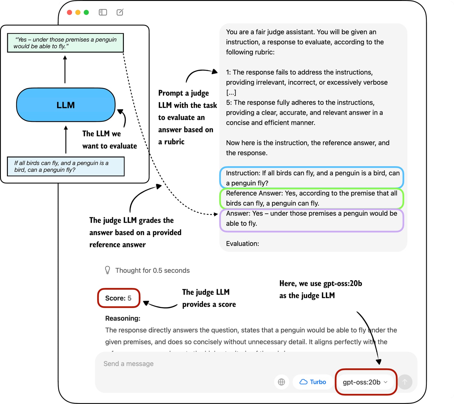
A related method is to use another LLM with a pre-defined grading rubric (i.e., an evaluation guide) to compare an LLM’s response to a reference response and judge the response quality based on a pre-defined rubric, as illustrated in Figure 12.
In practice, the judge-based approach shown in Figure 12 works well when the judge LLM is strong. Common setups use leading proprietary LLMs via an API (e.g., the GPT-5 API), though specialized judge models also exist. (E.g., one of the many examples is Phudge; ultimately, most of these specialized models are just smaller models fine-tuned to have similar scoring behavior as proprietary GPT models.)
One of the reasons why judges work so well is also that evaluating an answer is often easier than generating one.
To implement a judge-based model evaluation as shown in Figue 12 programmatically in Python, we could either load one of the larger Qwen3 models in PyTorch and prompt it with a grading rubric and the model answer we want to evaluate.
Alternatively, we can use other LLMs through an API, for example the ChatGPT or Ollama API.
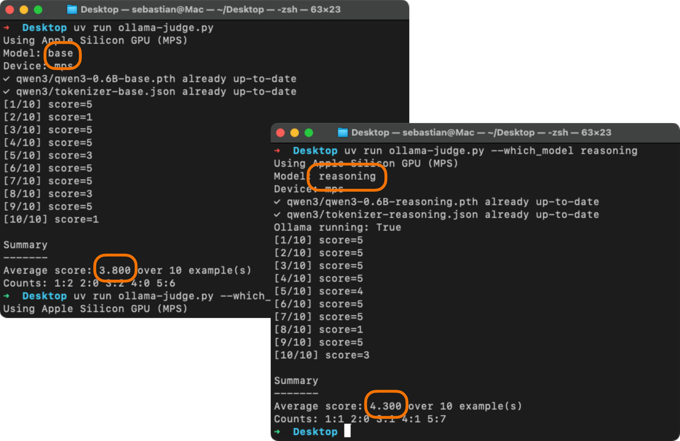
As we already know how to load Qwen3 models in PyTorch, to make it more interesting, in the remainder of the section, we will implement the judge-based evaluation shown in Figure 12 using the Ollama API in Python.
Specifically, we will use the 20-billion parameter gpt-oss open-weight model by OpenAI as it offers a good balance between capabilities and efficiency. For more information about gpt-oss, please see my From GPT-2 to gpt-oss: Analyzing the Architectural Advances article:
Ollama is an efficient open-source application for running LLMs on a laptop. It serves as a wrapper around the open-source llama.cpp library, which implements LLMs in pure C/C++ to maximize efficiency. However, note that Ollama is only a tool for generating text using LLMs (inference) and does not support training or fine-tuning LLMs.
To execute the following code, please install Ollama by visiting the official website at https://ollama.com and follow the provided instructions for your operating system:
For macOS and Windows users: Open the downloaded Ollama application. If prompted to install command-line usage, select “yes.”
For Linux users: Use the installation command available on the Ollama website.
Before implementing the model evaluation code, let’s first download the gpt-oss model and verify that Ollama is functioning correctly by using it from the command line terminal.
Execute the following command on the command line (not in a Python session) to try out the 20 billion parameter gpt-oss model:
ollama run gpt-oss:20bThe first time you execute this command, the 20 billion parameter gpt-oss model, which takes up 14 GB of storage space, will be automatically downloaded. The output looks as follows:
$ ollama run gpt-oss:20b pulling manifest pulling b112e727c6f1: 100% ▕██████████████████████▏ 13 GB pulling fa6710a93d78: 100% ▕██████████████████████▏ 7.2 KB pulling f60356777647: 100% ▕██████████████████████▏ 11 KB pulling d8ba2f9a17b3: 100% ▕██████████████████████▏ 18 B pulling 55c108d8e936: 100% ▕██████████████████████▏ 489 B verifying sha256 digest writing manifest removing unused layers successAlternative Ollama models
Note that the gpt-oss:20b in the ollama run gpt-oss:20b command refers to the 20 billion parameter gpt-oss model. Using Ollama with the gpt-oss:20b model requires approximately 13 GB of RAM. If your machine does not have sufficient RAM, you can try using a smaller model, such as the 4 billion parameter qwen3:4b model via ollama run qwen3:4b, which only requires around 4 GB of RAM.
For more powerful computers, you can also use the larger 120-billion parameter gpt-oss model by replacing gpt-oss:20b with gpt-oss:120b. However, keep in mind that this model requires significantly more computational resources.
Once the model download is complete, we are presented with a command-line interface that allows us to interact with the model. For example, try asking the model, “What is 1+2?”:
>>> What is 1+2? Thinking... User asks: “What is 1+2?” This is simple: answer 3. Provide explanation? Possibly ask for simple arithmetic. Provide answer: 3. ...done thinking. 1 + 2 = **3**You can end this ollama run gpt-oss:20b session using the input /bye.
You can end this ollama run gpt-oss:20b session using the input /bye.
In the remainder of this section, we will use the ollama API. This approach requires that Ollama is running in the background. There are three different options to achieve this:
1. Run the ollama serve command in the terminal (recommended). This runs the Ollama backend as a server, usually on http://localhost:11434. Note that it doesn’t load a model until it’s called through the API (later in this section).
2. Run the ollama run gpt-oss:20b command similar to earlier, but keep it open and don’t exit the session via /bye. As discussed earlier, this opens a minimal convenience wrapper around a local Ollama server. Behind the scenes, it uses the same server API as ollama serve.
3. Ollama desktop app. Opening the desktop app runs the same backend automatically and provides a graphical interface on top of it as shown in Figure 12 earlier.
Ollama server IP address
Ollama runs locally on our machine by starting a local server-like process. When running ollama serve in the terminal, as described above, you may encounter an error message saying Error: listen tcp 127.0.0.1:11434: bind: address already in use.
If that’s the case, try use the command OLLAMA_HOST=127.0.0.1:11435 ollama serve (and if this address is also in use, try to increment the numbers by one until you find an address not in use.)
The following code verifies that the Ollama session is running properly before we use Ollama to evaluate the test set responses generated in the previous section:
import psutil def check_if_running(process_name): running = False for proc in psutil.process_iter(["name"]): if process_name in proc.info["name"]: running = True break return running ollama_running = check_if_running("ollama") if not ollama_running: raise RuntimeError( "Ollama not running. " "Launch ollama before proceeding." ) print("Ollama running:", check_if_running("ollama"))Ensure that the output from executing the previous code displays Ollama running: True. If it shows False, please verify that the ollama serve command or the Ollama application is actively running (see Figure 13).
In the remainder of this article, we will interact with the local gpt-oss model, running on our machine, through the Ollama REST API using Python. The following query_model function demonstrates how to use the API:
import json import urllib.request def query_model( prompt, model="gpt-oss:20b", # If you used # OLLAMA_HOST=127.0.0.1:11435 ollama serve # update the address below url="http://localhost:11434/api/chat" ): # Create the data payload as a dictionary: data = { "model": model, "messages": [ {"role": "user", "content": prompt} ], # Settings required for deterministic responses: "options": { "seed": 123, "temperature": 0, "num_ctx": 2048 } } # Convert the dictionary to JSON and encode it to bytes payload = json.dumps(data).encode("utf-8") # Create a POST request and add headers request = urllib.request.Request( url, data=payload, method="POST" ) request.add_header("Content-Type", "application/json") response_data = "" # Send the request and capture the streaming response with urllib.request.urlopen(request) as response: while True: line = response.readline().decode("utf-8") if not line: break # Parse each line into JSON response_json = json.loads(line) response_data += response_json["message"]["content"] return response_dataHere’s an example of how to use the query_model function that we just implemented:
ollama_model = "gpt-oss:20b" result = query_model("What is 1+2?", ollama_model) print(result)The resulting response is “3”. (It differs from what we’d get if we ran Ollama run or the Ollama application due to different default settings.)
Using the query_model function, we can evaluate the responses generated by our model with a prompt that includes a grading rubric asking the gpt-oss model to rate our target model’s responses on a scale from 1 to 5 based on a correct answer as a reference.
The prompt we use for this is shown below:
def rubric_prompt(instruction, reference_answer, model_answer): rubric = ( "You are a fair judge assistant. You will be " "given an instruction, a reference answer, and " "a candidate answer to evaluate, according to " "the following rubric:\n\n" "1: The response fails to address the " "instruction, providing irrelevant, incorrect, " "or excessively verbose content.\n" "2: The response partially addresses the " "instruction but contains major errors, " "omissions, or irrelevant details.\n" "3: The response addresses the instruction to " "some degree but is incomplete, partially " "correct, or unclear in places.\n" "4: The response mostly adheres to the " "instruction, with only minor errors, " "omissions, or lack of clarity.\n" "5: The response fully adheres to the " "instruction, providing a clear, accurate, and " "relevant answer in a concise and efficient " "manner.\n\n" "Now here is the instruction, the reference " "answer, and the response.\n" ) prompt = ( f"{rubric}\n" f"Instruction:\n{instruction}\n\n" f"Reference Answer:\n{reference_answer}\n\n" f"Answer:\n{model_answer}\n\n" f"Evaluation: " ) return promptThe model_answer in the rubric_prompt is intended to represent the response produced by our own model in practice. For illustration purposes, we hardcode a plausible model answer here rather than generating it dynamically. (However, feel free to use the Qwen3 model we loaded at the beginning of this article to generate a real model_answer).
Next, let’s generate the rendered prompt for the Ollama model:
rendered_prompt = rubric_prompt( instruction=( "If all birds can fly, and a penguin is a bird, " "can a penguin fly?" ), reference_answer=( "Yes, according to the premise that all birds can fly, " "a penguin can fly." ), model_answer=( "Yes – under those premises a penguin would be able to fly." ) ) print(rendered_prompt)The output is as follows:
You are a fair judge assistant. You will be given an instruction, a reference answer, and a candidate answer to evaluate, according to the following rubric: 1: The response fails to address the instruction, providing irrelevant, incorrect, or excessively verbose content. 2: The response partially addresses the instruction but contains major errors, omissions, or irrelevant details. 3: The response addresses the instruction to some degree but is incomplete, partially correct, or unclear in places. 4: The response mostly adheres to the instruction, with only minor errors, omissions, or lack of clarity. 5: The response fully adheres to the instruction, providing a clear, accurate, and relevant answer in a concise and efficient manner. Now here is the instruction, the reference answer, and the response. Instruction: If all birds can fly, and a penguin is a bird, can a penguin fly? Reference Answer: Yes, according to the premise that all birds can fly, a penguin can fly. Answer: Yes – under those premises a penguin would be able to fly. Evaluation:Ending the prompt in “Evaluation: “ incentivizes the model to generate the answer. Let’s see how the gpt-oss:20b model judges the response:
result = query_model(rendered_prompt, ollama_model) print(result)The response is as follows:
**Score: 5** The candidate answer directly addresses the question, correctly applies the given premises, and concisely states that a penguin would be able to fly. It is accurate, relevant, and clear.As we can see, the answer receives the highest score, which is reasonable, as it is indeed correct. While this was a simple example stepping through the process manually, we could take this idea further and implement a for-loop that iteratively queries the model (for example, the Qwen3 model we loaded earlier) with questions from an evaluation dataset and evaluate it via gpt-oss and calculate the average score. You can find an implementation of such a script where we evaluate the Qwen3 model on the MATH-500 dataset here on GitHub.
Scoring intermediate reasoning steps with process reward models
Related to symbolic verifiers and LLM judges, there is a class of learned models called process reward models (PRMs). Like judges, PRMs can evaluate reasoning traces beyond just the final answer, but unlike general judges, they focus specifically on the intermediate steps of reasoning. And unlike verifiers, which check correctness symbolically and usually only at the outcome level, PRMs provide step-by-step reward signals during training in reinforcement learning. We can categorize PRMs as “step-level judges,” which are predominantly developed for training, not pure evaluation. (In practice, PRMs are difficult to train reliably at scale. For example, DeepSeek R1 did not adopt PRMs and instead combined verifiers for the reasoning training.)
Judge-based evaluations offer advantages over preference-based leaderboards, including scalability and consistency, as they do not rely on large pools of human voters. (Technically, it is possible to outsource the preference-based rating behind leaderboards to LLM judges as well). However, LLM judges also share similar weaknesses with human voters: results can be biased by model preferences, prompt design, and answer style. Also, there is a strong dependency on the choice of judge model and rubric, and they lack the reproducibility of fixed benchmarks.
In this article, we covered four different evaluation approaches: multiple choice, verifiers, leaderboards, and LLM judges.
I know this was a long article, but I hope you found it useful for getting an overview of how LLMs are evaluated. A from-scratch approach like this can be verbose, but it is a great way to understand how these methods work under the hood, which in turn helps us identify weaknesses and areas for improvement.
That being said, you are probably wondering, “What is the best way to evaluate an LLM?” Unfortunately, there is no single best method since, as we have seen, each comes with different trade-offs. In short:
Multiple-choice
(+) Relatively quick and cheap to run at scale
(+) Standardized and reproducible across papers (or model cards)
(-) Measures basic knowledge recall
(-) Does not reflect how LLMs are used in the real world
Verifiers
(+) Standardized, objective grading for domains with ground truth
(+) Allows free-form answers (with some constraints on final answer formatting)
(+) Can also score intermediate steps if using process verifiers or process reward models
(-) Requires verifiable domains (for example, math or code), and building good verifiers can be tricky
(-) Outcome-only verifiers evaluate only the final answer, not reasoning quality
Arena-style leaderboards (human pairwise preference)
(+) Directly answers “Which model do people prefer?” on real prompts
(+) Allows free-form answers and implicitly accounts for style, helpfulness, and safety
(-) Expensive and time-intensive for humans
(-) Does not measure correctness, only preference
(-) Nonstationary populations can affect stability
LLM-as-a-judge
(+) Scalable across many tasks
(+) Allows free-form answers
(-) Dependent on the judge’s capability (ensembles can make this more robust)
(-) Depends on rubric choice
While I am usually not a big fan of radar plots, one can be helpful here to visualize these different evaluation areas, as shown below.
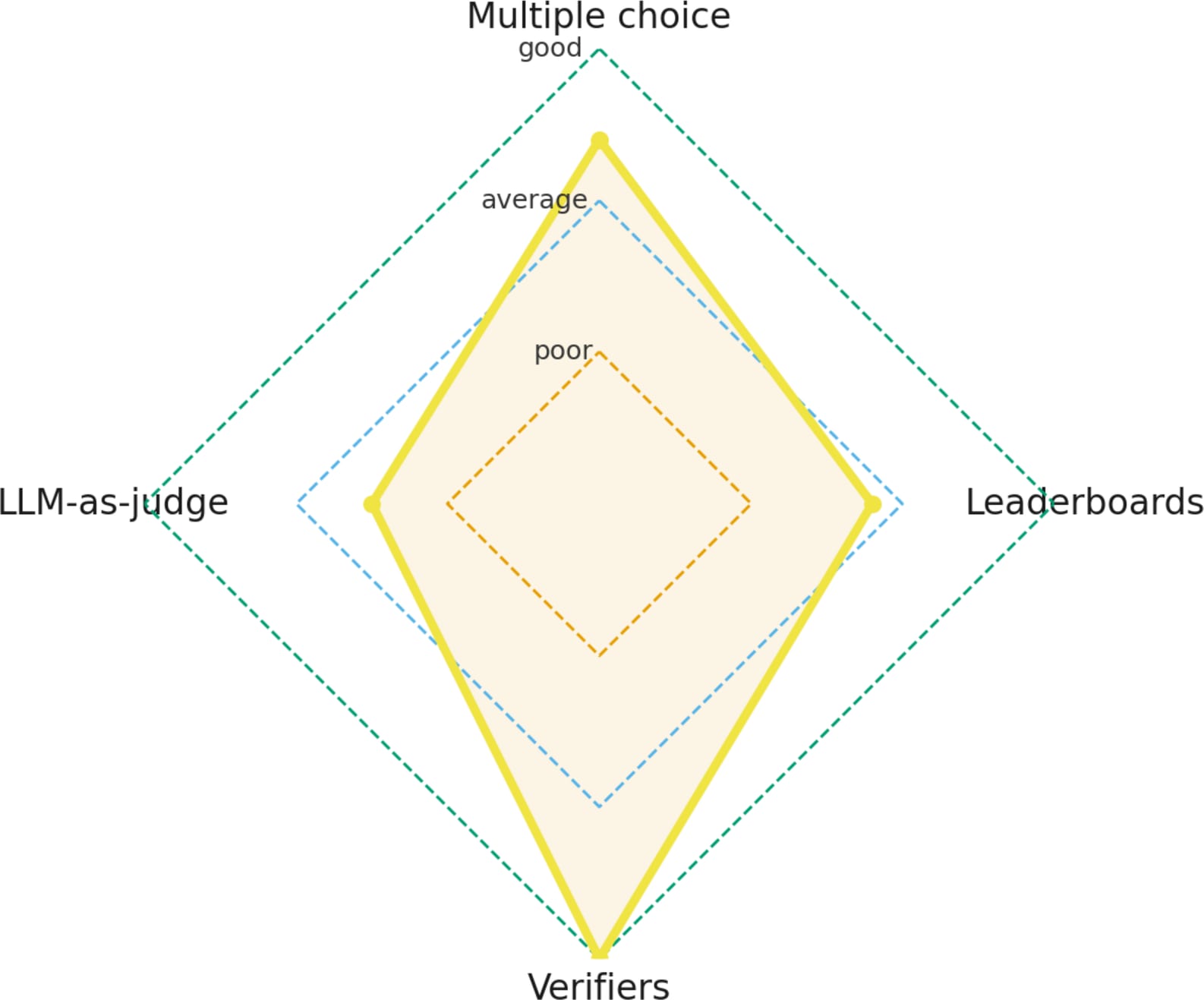
For instance, a strong multiple-choice rating suggests that the model has solid general knowledge. Combine that with a strong verifier score, and the model is likely also answering technical questions correctly. However, if the model performs poorly on LLM-as-a-judge and leaderboard evaluations, it may struggle to write or articulate responses effectively and could benefit from some RLHF.
So, the best evaluation combines multiple areas. But ideally it also uses data that directly aligns with your goals or business problems. For example, suppose you are implementing an LLM to assist with legal or law-related tasks. It makes sense to run the model on standard benchmarks like MMLU as a quick sanity check, but ultimately you will want to tailor the evaluations to your target domain, such as law. You can find public benchmarks online that serve as good starting points, but in the end, you will want to test with your own proprietary data. Only then can you be reasonably confident that the model has not already seen the test data during training.
In any case, model evaluation is a very big and important topic. I hope this article was useful in explaining how the main approaches work, and that you took away a few useful insights for the next time you look at model evaluations or run them yourself.
As always,
Happy tinkering!
This magazine is a personal passion project, and your support helps keep it alive.
If you’d like to support my work, please consider my Build a Large Language Model (From Scratch) book or its follow-up, Build a Reasoning Model (From Scratch). (I’m confident you’ll get a lot out of these; they explain how LLMs work in depth you won’t find elsewhere.)
Thanks for reading, and for helping support independent research!
If you read the book and have a few minutes to spare, I’d really appreciate a brief review. It helps us authors a lot!
Your support means a great deal! Thank you!