.png)

This post is part of a series of paper reviews, covering the ~30 papers Ilya Sutskever sent to John Carmack to learn about AI. To see the rest of the reviews, go here.
In 2019, AI researcher and co-founder of modern RL Rich Sutton posted a diary entry that has since become famous in data science, computer science, and ML/AI. The post is titled "The Bitter Lesson":
We have to learn the bitter lesson that building in how we think we think does not work in the long run. The bitter lesson is based on the historical observations that 1) AI researchers have often tried to build knowledge into their agents, 2) this always helps in the short term, and is personally satisfying to the researcher, but 3) in the long run it plateaus and even inhibits further progress, and 4) breakthrough progress eventually arrives by an opposing approach based on scaling computation by search and learning. The eventual success is tinged with bitterness, and often incompletely digested, because it is success over a favored, human-centric approach.
The pattern that Sutton lays out appears in chess, in Go, in computer vision…basically any area that has ever been touched by machine learning. As a result, there is an entire class of papers that I call "bitter lesson" papers. These are publications that basically come into a pre-existing field and say "hey, love all of the stuff you guys were doing before, it's real cool and all, but we're doing neural networks now." The AlexNet paper, when neural networks first beat heuristics-based models on the ImageNet segmentation task, is a 'bitter lesson' paper. The AlphaFold paper, when neural networks first beat heuristics-based models on protein folding, is a 'bitter lesson' paper. And Deep Speech 2 (DS2), published in 2015, is a 'bitter lesson' paper.
The authors aim to apply the bitter lesson towards speech recognition (also known as speech-to-text). They aren't subtle about their intentions. Here is how DS2 opens:
Decades worth of hand-engineered domain knowledge has gone into current state-of-the-art automatic speech recognition (ASR) pipelines. A simple but powerful alternative solution is to train such ASR models end-to-end, using deep learning to replace most modules with a single model [26].
ASR is an interesting problem space. Audio as a modality is extremely complex and hard to work with. Like video, there are strong temporal dependencies. But unlike video, there is no easy way to discretize audio through sampling. Spoken words do not follow any obvious patterns that can be exploited to make the data easier to work with. Add in variability in acoustics, pronunciation, background noise, and input/output length, and you have the makings of a seemingly intractable problem. Live-streaming makes this all worse — in addition to the above, you also have to deal with consumer-tolerable latencies to make a reasonable product experience.
Historically, the solution was to try and apply human expertise — that is, build out a bunch of modules that try to figure out what is happening in an audio track through comprehensive hand-made heuristics. "There are 44 phonemes in the English language, try to map each sound to a phoneme and then work backwards to figure out the words being used" things like that. And some approaches from 2013 and 2014 use deep neural networks in modular ways, as part of larger systems, e.g. to do the mapping between particular samples of audio and phonemes.
The authors of Deep Speech 2 throw all that out and replace it with a big neural net.
DS2 is, as a result, a scaling paper and an engineering paper. Following in the tradition of AlexNet, DS2 is essentially a grab-bag of engineering tricks to get the neural net to work. There is no attempt at presenting a theory for why the system works. Nor is there any complex analogizing to physics / neuroscience / mathematics. Rather, the paper is a collection of tips for practitioners about how to get large models with a lot of data to do the right thing.
The nature of this paper makes it difficult to construct any overarching narrative. I'm going to try to cover most of the important highlights in quick succession, but treat this more like an index and cntrl-f the paper to dive deeper into areas of more interest. There are three sections, focusing on the underlying model, the training process, and the real-world deployment respectively. Each section is a grab bag of topics, some big and some small.
Note that the paper discusses training models for both English and Mandarin, but since the overall construction is basically the same for both I'll just shorthand to discussing the English variant.
Architecture. Input waveforms are represented as spectrogram images, and outputs are represented as RNN-decoded characters (26 characters of the alphabet plus space, apostrophe, and blank) one per 'timestep'. The authors start with several convolutional layers to embed the spectrogram, followed by a stack of bi-directional RNNs, followed by a fully connected layer with a softmax on top. The bi-directional RNNs allow each intermediate token embedding to take in information about its previous context and its future context, as in link. You can think of them as a primitive transformer — each token gets some amount of information about every other token in the sequence (it just cannot attend to only those tokens that are important). The authors experiment with a few different numbers of layers and find that bigger is better. The one additional interesting note is that they use a clipped ReLU, where activations are not allowed to go higher than 20. This is likely as a stability measure to prevent spiking gradients — we'll see this again when we discuss batch norm a bit further down.
Loss. The authors use a "connectionist temporal classification" (CTC) loss, something I had never heard of before this paper. ASR as a problem area is difficult because there is no guaranteed single alignment between a given audio sample and a speech output.
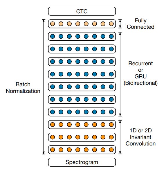
Imagine I had an audio clip of the word 'hello'. We have to discretize this clip in some way to eventually output individual character tokens. Naively, we could chunk the audio waveform. But there is no way to guarantee that you will chunk your data in a way that lands exactly where a character would be. That doesn't even make sense, we don't pronounce most characters! So if the model outputs -h-e-ll-o- or hh-e-ll-oo or -hel-lo-- (where the - dash represents a 'blank', i.e. no character output at that timestep), we need to treat these all as 'correct' in some way in whatever loss function we end up with.
In DS2, at each timestep, we get a probability distribution over all symbols (including the blank). So at timestep t, you have a total of t probability vectors output by the model that represent different possible character sequences. The CTC loss sums all of the probability sequences that lead to the right text output. So, for example, the first character should be represented by a probability vector like the one below:

There's some weight on the H token and some on the blank token, and that's it — those are the only two possible valid starting points. We then sum that with the next vector, which can either be H, E, or blank. And so on. Maximizing the sum of these possible outcomes is equivalent to training the model to do unaligned transcription. (Naively, this loss is expensive to calculate, but luckily it turns out there is a simple dynamic programming approach that dramatically reduces the complexity of computing the loss)
Batch norm. In 2015, we didn't really know how to make models really big. One issue was gradient instability during training.
Neural networks are trained with back propagation, which is an algorithm that calculates partial gradients for each weight in a neural network. In deep networks, weights in early layers often receive very small gradients during backpropagation, making them hard to train — or sometimes effectively ignored. Or, sometimes, small changes in early weights are amplified through the layers, making them unstable.
In many early model architectures, gradients are multiplicatively composed across layers. If each layer causes even a slight amplification or attenuation of the gradient, the effect compounds, potentially leading to exploding or vanishing gradients. In both cases, training will basically hit a dead end. Once a model starts to behave erratically, it is very difficult to get it back on track towards learning useful things. Larger models are much more susceptible to this problem, because the gradient multiplication effects are more severe for each additional layer.
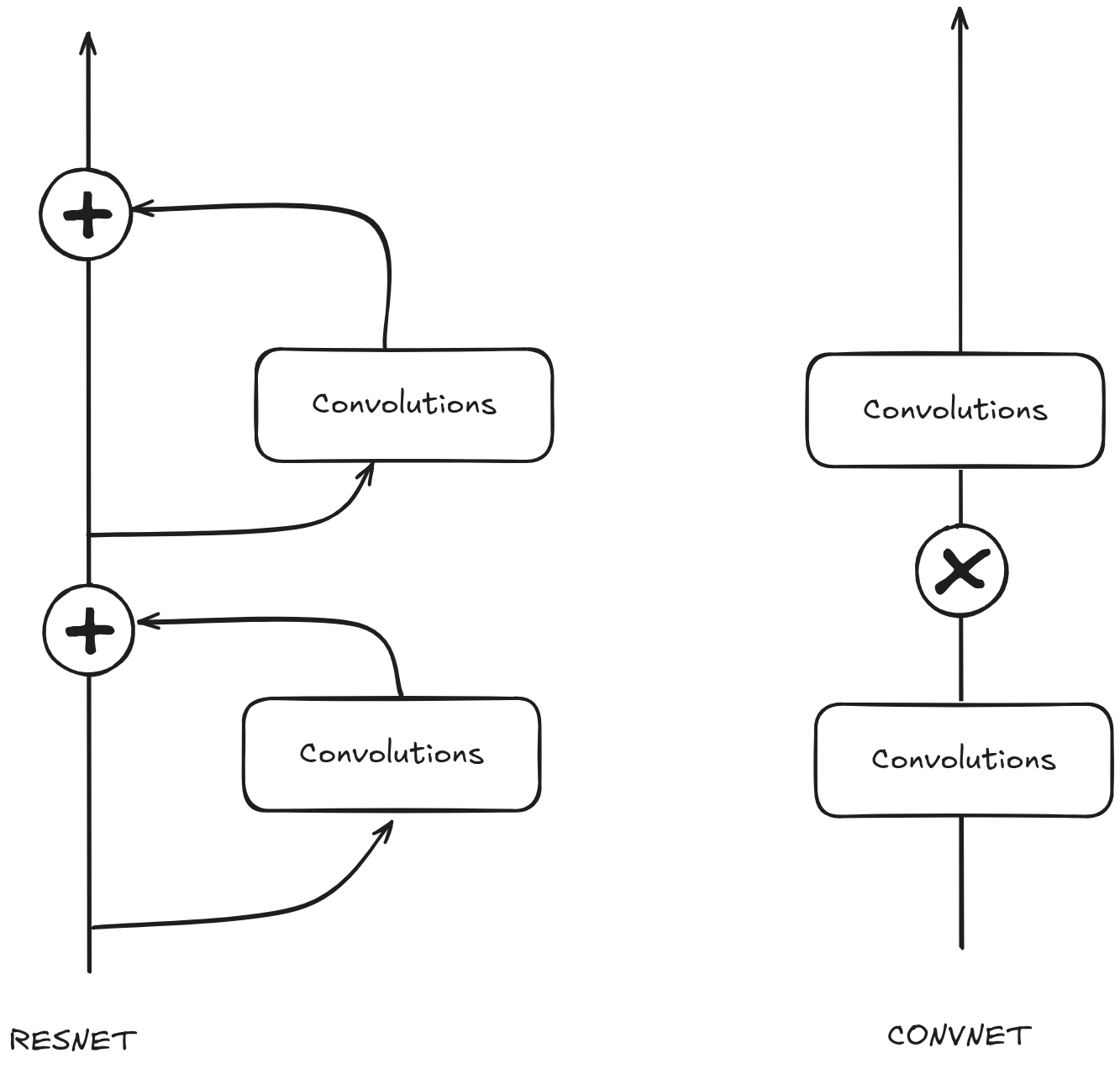
We've seen this issue before. LSTMs and ResNets both attempt to solve this problem by making successive layers additive instead of multiplicative.
But there are other ways to mitigate this issue. One way is by clipping the ReLU activations — we briefly mentioned that above. The basic idea is that you just prevent training from ever becoming unstable by preventing weights from getting too large to begin with.
Another way is by reducing sources of instability.
In an ideal setting, you would train a neural network on an entire training dataset at once. Unfortunately most useful datasets are way too big to load into memory. So instead, we randomize the dataset, batch it, and hope that the model converges to the same place that it would if we didn't have to batch the data. In theory, if there were no limits on time or resources, batched "stochastic" gradient descent would eventually behave the same as regular full dataset gradient descent. In practice, randomness can cause problems.
Imagine you were training an animal image classifier, and the first batch was all images of dogs (It's unlikely, but not impossible for this to occur depending on your dataset). Your model would overfit on dogs. It may decide that dogs are obviously the most important thing. And it may end up dropping gradients to 0 for all future batches, especially if the learning rate decreases in tandem. Or, alternatively, if your model hits that batch in the middle of training, it may suddenly get super strong gradients pointing in the "dog" direction, and start swinging wildly all over the place until the system falls apart.
You can reduce some of this effect by calculating batch-specific statistics like the mean and standard deviation, and then normalizing the data in the batch so that the variation in the activations and gradients isn't so intense. If a particular batch comes in that is extremely variable, the "batch norm" will reduce that variation and smooth out training. This is not the first paper to ever use batch norm. Prior work showed that batch norm was useful for speeding up training, so it was around. But DS2 may be the paper that popularized its usage for model scaling. The authors convincingly argue that batch norm was critical both for speeding up training and for improving model generalization.
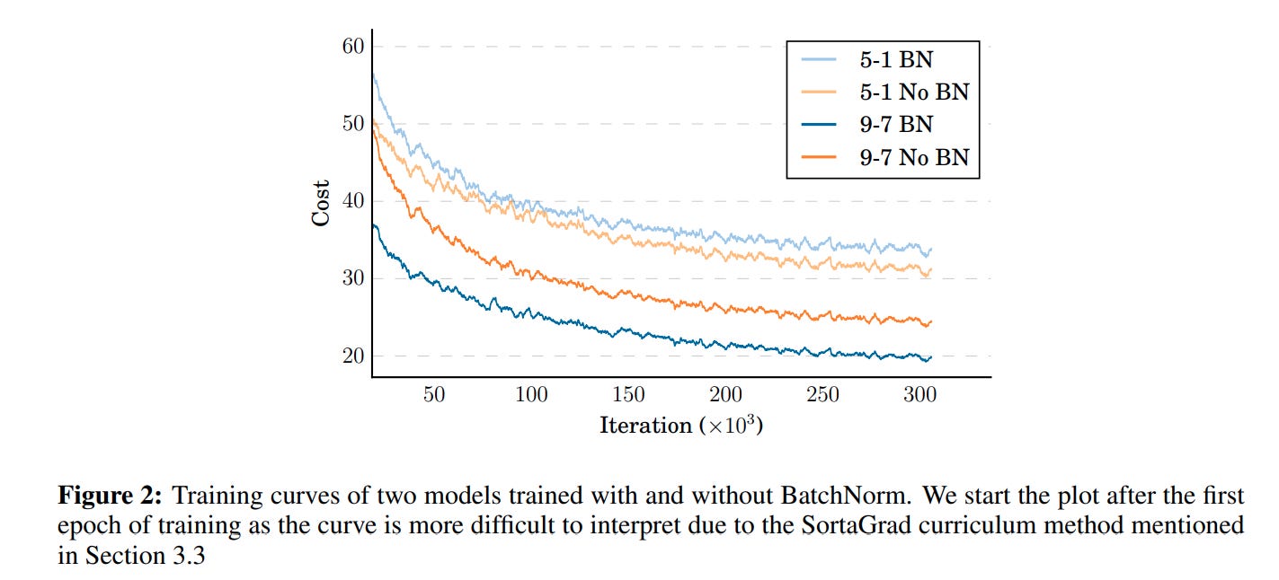
This is also the first paper to show how to effectively deploy batch norm layers at inference time. Previously, this was a difficult problem — batch statistics only really work if you have a batch. Models trained with batch norm that do not use batched inference end up performing significantly worse, because the layers are all calibrated incorrectly. ASR is an example of a scenario where you will definitely have inputs that need to be processed on demand in real time, i.e. batch size = 1. To solve this problem, the authors keep rolling averages of the mean and stddev, and simply apply those at inference time on all incoming data instead of calculating new batch statistics on the fly. This has become standard practice for all modern day batch norm implementations, as far as I'm aware.
SortaGrad. Everyone knows what batch norm is. Incredibly popular technique, required reading for practitioners (though it has mostly been replaced by LayerNorm), especially if you want to learn anything about ML from 2015 to 2020. By contrast, I don't think anyone knows what Sortagrad is. Or at least, this paper is the first I've heard of it. And a quick Google Search suggests it's also the last paper to use it. use this particular learning strategy.
The basic idea is that the CTC loss described above is a function of the length of the input audio sample. The input can be variable length, and the CTC loss will basically always be higher for longer inputs than shorter ones. Intuitively, this is because the CTC loss sums over all of the valid alignment possibilities, which become exponentially larger the more audio there is.
SortaGrad is a learning curriculum that orders the training data such that the model sees shorter audio samples first, before eventually moving to longer ones. It's not a particularly crazy idea, as far as learning curricula go — the same basic idea has been applied to text and to image gen, the latter most famously in NVIDIA's GAN papers. The authors note that SortaGrad improves training speeds and reduces numerical instability, the latter because larger audio samples will have higher gradients (which, as we discussed earlier, is bad). I think learning curricula in general have become more important, especially in the diffusion world. In general, starting small and scaling up seems to work better than pure randomization.
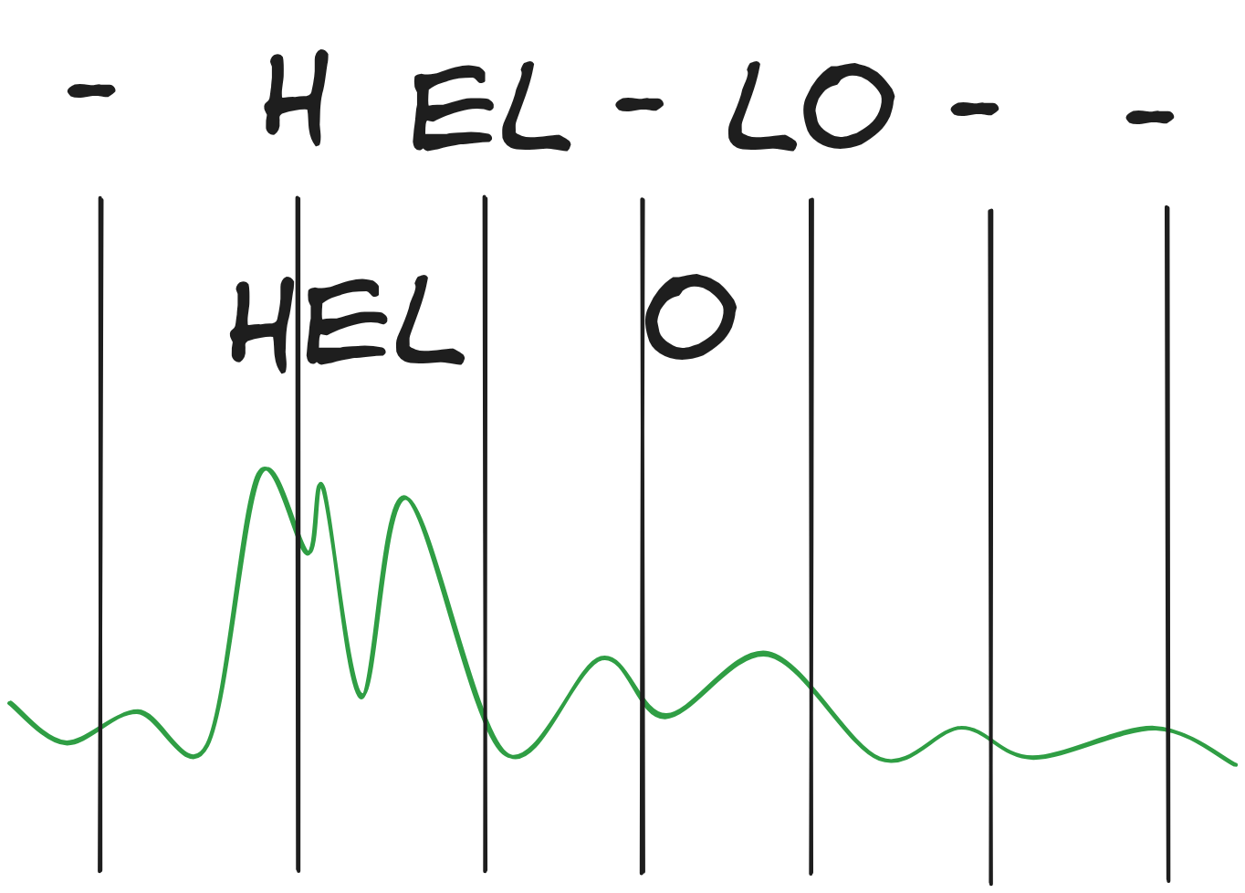
Convolutions. The input audio sample is converted to a spectrogram. If you've never seen one of those, it looks like this:
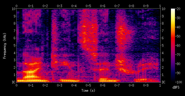
The x-axis is time, the y-axis is frequency. From a neural network perspective, a spectrogram is basically an image. Pixels have the same general geospatial locality constraints in spectrograms as they do in any other image. So, as you might expect, you can run a convolutional network over a spectrogram and get pretty good results.
The authors experiment with a few variations of convolutional layers — 1D (only in the time), 2D (in both time and frequency), and with strides.
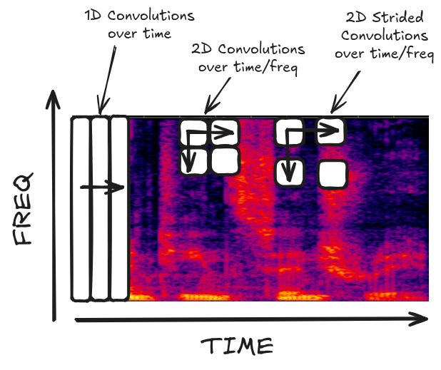
You can think of striding as a form of sampling the input. Striding strictly makes the model worse, but it dramatically speeds up training and reduces resource usage by lowering the size of the input. However, they have a small problem: their output model is spitting out characters and requires at least one input timestep per output character. But many words in English have multiple characters in the same part of the audio. The word "squirrelled" has 11 characters, but is pronounced in a single syllable! If you accidentally stride over that part of the audio sample, you're going to miss a lot of outputs.
The authors get around this by expanding their output vocabulary into something that resembles the modern day transformer 'tokens' that we are more familiar with. They take non-overlapping bigrams and transform the existing single-character labels into ones that can be parsed as multi-character labels. For example, "the sentence the cat sat with non-overlapping bigrams is segmented as [th, e, space, ca,t, space, sa,t]." This has the added benefit of reducing the length of the output transcription, thereby saving a bit on processing time and memory.
Row convolutions. Before we mentioned that batch norm doesn't quite work right at inference time, where you may not have 'batches' of data to calculate statistics. It turns out bi-directional RNN's have a similar problem. The point of a bidirectional RNN is for every token to have the full context of a sentence — both the context of everything leading up to the given token, and the context for everything coming after. But, like, in a real time transcription setting, you don't have the stuff that comes after! How do these things work during inference time?
The authors propose a new kind of layer they call "Row Convolution." The basic idea is that you do not actually need all of the context in order to do character transcription, just the next few timesteps. So they cap the 'backwards pass' of the bidirectional RNN to something that looks like this:
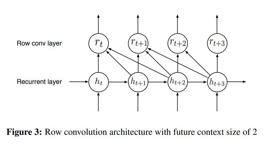
This model works about as well as their original model, and of course is much more useful in online settings.
N-gram modelling. The DS2 model is learning speech to text, but that doesn't necessarily mean it should learn how to handle homophones. Like, strictly speaking, the model could learn to output 'to' instead of 'two', as in 'to plus to equals four'. Even though it is obviously wrong, it is phonetically correct, so we may expect the model to regularly screw up on inputs like this. But the model does not do this, or at least not with the frequency we would expect. It seems that there are many cases where the model correctly figures out what words to use based on the context around it. In other words, this model — which is only being trained to learn speech to text — implicitly learns a language model too.
It's not, like, a particularly good language model though. The DS2 model is trained over millions of audio samples, but most pure language models, even back in 2015, were trained over hundreds of millions of lines of text. This raises the obvious question: can you improve DS2 by pairing it with an explicit language model?
The authors train an n-gram language model on 250 million lines from Common Crawl (i.e. internet scrapes). During inference, they take the output transcription probabilities from their model and search for the transcription that maximizes both the CTC trained network's predicted output AND the language model's predicted output. Note that it's unlikely that the language model is doing any significant lifting through actual token prediction. Rather, it helps the model with things like spelling mistakes. But, still, this is exactly the kind of real-world combination that leverages the best of deep learning with the best of algorithmic approaches.
So at this point we've described all of the various modelling bits and pieces that these guys did to get DS2 off the ground. But we're not out of the woods yet — in 2015, training models with tens of millions of parameters was pretty difficult! So next up, we'll dive into some of the approaches the authors used to make training more effective.
Training parallelism. If you have a bunch of GPUs, how do you best utilize those GPUs to improve your model?
One approach — especially popular in the modern era, especially if you have a ton of data — is to simply make a bigger model. You can split your weights across many of the GPUs, and run a forward pass using all of your GPUs at once. If you have 8 GPUs, you can make a model that is 8x bigger than if you had only 1 GPU. AlexNet did this reasonably effectively by doubling their model size across two GPUs. GPIPE did this by splitting models 'vertically' by layer and putting each chunk of layers onto individual GPUs. And the larger AI assistants — Claude, Gemini, GPT — split models 'horizontally' as well, by putting a single really big layer across many GPUs at once.
But back in 2015, we didn't really know how to make really big models (that's kind of what the DS2 paper is about!) and we also didn't really have the data to justify it. So making a bigger model isn't super relevant for the authors, who are already making a pretty big model for the time period.
Ok, but you still have all these GPUs. What else?
Another approach is to parallelize your training. You could instantiate the same model across a bunch of different GPUs, and then send a mini-batch of data to each one. This effectively lets you train across N batches at the same time. So if I have 8 GPUs, and my model fits on a single GPU, I can speed up training by 8x. This is obviously useful regardless of model size.
When parallelizing batches, you have a choice: you can run each batch independent of all the rest of the batches, collecting gradients from each model and applying them as they come in; or you can run each batch together with all of the rest of the batches, and wait for each batch to finish before moving onto the next one. The former is known as 'synchronous' training, and the latter as asynchronous.
The basic trade-off here is speed vs. accuracy. Anyone who has ever worked with distributed computing knows that the speed of your system is beholden to your slowest node. If you have a bunch of workers processing data, and you need to synchronize all of them before you can move to the next step, your network is as slow as your slowest worker. In theory they should all be roughly the same speed; in practice, network latency, hardware latency, and general randomness can slow things down a lot. On the flip side, if you let all of your workers run without waiting for the others, you may end up in a situation where your model is getting 'stale' results from a worker that has for some reason lagged way behind. This staleness is another potential source of instability, which, as discussed above, is really dangerous in large models. And the asynchronous mode has the additional flaw of being non-deterministic, which can be quite frustrating if you are debugging.
Picture
The authors use synchronous gradient descent. They parallelize batches across a bunch of GPUs and wait for each one to finish. Then they sum up the gradients across the different workers, and apply those gradients to all of the models simultaneously before continuing.
Custom implementations. I don't really have an interest in really going in detail on code, but it's worth mentioning in passing: the authors wrote a bunch of custom code kernels and low level processes to really optimize their models. In addition to a custom GPU implementation of the CTC loss that makes use of a custom all-reduce implementation they also wrote a custom GPU memory allocator. The default allocator, cudaMalloc, is primarily optimized for multiple processes sharing memory resources. For DS2, there is only ever one process, so they can remove a bunch of overhead by simply preallocating all GPU memory at the start of training.
One interesting note: the authors point out that in many cases, GPU memory is used primarily for layer activations instead of for model parameters. In other words, if you have a really long input audio sample, the model may run out of memory. But if you design your model to handle those really long input audio samples, you are leaving some GPU allocation on the floor in the average case. Put another way, if you expect that most of the time you won't get really long audio samples, you can squeeze a bit more juice out of your GPUs by creating a bigger model. The authors design their memory allocator to handle outliers so that things don't crash when they get really long inputs. This, in turn, makes the model better on average everywhere else.
Dataset creation and augmentation. I've said in my Tech Things posts that data is a key driver for getting better models. Unsurprisingly, a paper about making really big models cares a lot about getting a ton of data. The authors collected thousands of hours of audio clips ranging from minutes to hours along with their noisy transcriptions, and then built a pipeline to turn that all into usable text aligned training samples.
For the most part, the pipeline is rather mundane — they segment the audio into chunks and remove audio clips that are too noisy or where the data can't be aligned at all. What I find most interesting is the first step of the pipeline: the authors use a preexisting bidirectional RNN trained with CTC to align the noisy transcription with the audio frames. That is, DS2 is trained by using smarter sampling from a weaker model. This is very similar to the training scheme I described in Deep Learning is Applied Topology:
Once they have their initial dataset, they augment the data by adding background noise, increasing their effective data samples while improving the model's overall robustness.
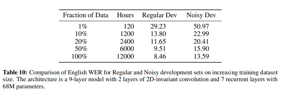
The authors note that model accuracy improves "by ~40% relative for each factor of 10 increase in the training set size." This is possibly the first power-law explicitly described in the neural network literature. We'll see more of this in the 2020 Scaling Laws paper, coming up.
DS2 isn't just a research paper. It is also a description of a real-world product. Like I said at the beginning, this paper is much more about engineering in practice than it is about academic benchmarks or abstract theory. So, of course, the authors spend the final chunk of the paper discussing how they actually went about deploying this thing in the real world. The highlights below.
Batch dispatch. Any real world consumer system has to deal with the fact that most consumers are impatient jerks who have the attention span of a flea. Latency is the name of the game — you have to make sure your system is fast, or no one will use it.
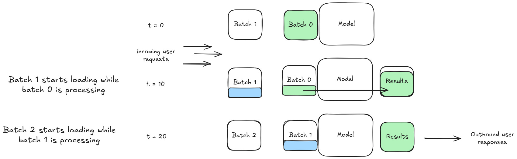
The DS2 folks have a small problem. They are serving their model on the web — of course — and most web servers are designed to handle multiple requests on different threads. This works great for standard CRUD apps. Different people can read or write to databases and overall have their requests handled efficiently without any latency at all. But the 'single thread per request' approach falls off a cliff when you have a GPU system that depends on having batches of data for maximum efficiency. You can't, like, wait around for a batch to be full before you send off a data request. That could take forever! But the alternative also doesn't work — if you only process data one audio input at a time, you'll build up a big backlog. Remember, the model is pretty big, and is designed to take up basically all of the GPU memory. If you get a big uptick in data all at once, and process them one at a time, you'll be wasting a bunch of GPU cycles while increasing end-user latency.
To get around this, the authors propose an algorithm called 'batch dispatch'. The basic idea is that while the model is in use, any incoming data will be stored in a batch. As soon as the model is done, the next batch is triggered and the process repeats. The batches are never completely full, so the GPUs are never utilized at 100% capacity. But this approach seems to cut a good throughline for minimizing the worst-case user latency experience.
Precision. Most papers are lucky if they have just one idea that becomes standard practice. This paper has at least two.
Computers represent numbers in a funny way. Let's say you had a fraction that repeats forever — say, 1/9, which in decimal is 0.1111… A computer can't represent that number with an infinite number of 1s. It has to cut off the number at some point. And in fact, it won't necessarily cut it off in precisely the same way across different machines, programming languages, compilers, architectures, and chips. Many modern systems are designed with 32-bit precision. That means that a number can be represented with up to 32-bits of data. Each bit is a 0 or a 1, so in binary 32-bits could represent numbers as large as 4294967296. In practice, you get a few bits less than that. There are normally only 7 significant figures that can be represented.
This may seem rather esoteric, but it turns out that this all matters quite a bit in neural network training. Those small differences in precision can pretty dramatically change training stability. In general, during training, you want to be as precise with your numerical methods as possible. Unfortunately there's no free lunch. The increase in precision comes with a memory trade off. If every number in your model is represented with, say, 64 bits instead of 32 bits, you have effectively doubled your model size.
But during inference, the whole stability thing matters way less. The authors realize that they can effectively cut their model size in half by using 16-bit numeric representations. And, importantly, this does not seem to meaningfully change the actual accuracy of the model a ton. Smaller models means cheaper deployments means happier CFOs.
This technique is now known as model quantization.

It is an extremely effective way to get models for edge computing — neural networks that can run on watches or smartphones without having to deal with network latency or remote data storage. It is also popular in the open source community, for folks who want to run the latest and greatest models on consumer hardware.
In my initial review of the AlexNet paper, I skimmed over a lot of the tips and tricks that they used to get their model to work. AlexNet is, frankly, an old paper. And even though it is in many ways responsible for revitalizing interest in neural networks, that paper simply does not have that much value to a modern day practitioner. DS2, on the other hand, feels fairly modern, even though it's a decade old. Yes, many of the architectural choices are a bit dated — layer norm has overtaken batch norm, and transformers would be a much better choice than bi-directional RNNs — but many of the deployment and training stabilization techniques are still extremely relevant.
From a theory perspective, there were two parts of this paper that really stood out.
The first is the power-law relationship between training data and model performance. In 2015, there was still a fair bit of controversy about the scaling hypothesis — that is, the idea that models would continue to get better as the amount of training data and available compute scaled up. There was some amount of intuition that these models would do better, but no one had rigorously examined how much better. Was the relationship linear? Logarithmic? Exponential? How much juice could we expect to squeeze from an additional GPU? As far as I'm aware, DS2 is the first time anyone showed rigorous results on the subject in an actual production setting. In 2025, the power-law relationship between training data and model performance is well established. In 2015, this was a key step towards inspiring a generation of researchers to build bigger.
The second is the idea of using a weaker model to train a newer, stronger model. Boosting has been around for a long time, so strictly speaking using weak models is not particularly new. But the particular implementation of sampling a weaker model to provide high quality training data for a new, stronger model that does more or less the exact same thing…I mean, that's basically what every AI shop in the world is doing these days. I don't know when exactly that approach became mainstream, but I was definitely surprised to see this strategy pop up as early as 2015.
Other than that, though, there's not much more to add. My insight section is a bit shorter than usual; at the end of the day, DS2 is an engineering paper, and the interesting bits are in the implementation, not in whatever fancy theory crafting I might do at the end.