.png)

Abstract
In a WeChat article titled How Large is the Phase Error of Commercially Available VNA Open and Short Calibration Kits? [1], a vendor claimed to have measured cheap, generic Vector Network Analyzer (VNA) calibration kits (“calkit”) commonly used in amateur radio, asserting they have errors of “tens, even hundreds of degrees.” However, the measurement data published by the vendor violates established principles of physics and engineering. To prevent this article from continuing to mislead readers, this article reveals the issues within the vendor’s data.
To facilitate understanding for readers without a background in RF/microwave measurement, this article first introduces the application and calibration principles of VNAs before detailing the problems. This article also includes numerous appendices, such as the SOL calculation algorithm, equivalent circuit models of calkits, and the parasitic parameters of coaxial opens/shorts, complete with source code. Beyond exposing the issues in the vendor’s article, this article can also serve as a primer and reference for academic literature on VNA calibration principles and coaxial parasitics calculations.
Note: Both the original WeChat article and this blog post were originally in Chinese, as a response to the misleading claims of a China-based vendor. Considering that the information is useful for the RF/microwave community in general, it is republished here in English. The source article contains more than 60,000 characters - an impractical translation workload for the author, thus machine translation has been used. This translation was generated by DeepSeek V3.1, with manual copyediting.
Background
Network Analyzer Calibration
In radio and microwave engineering, the Vector Network Analyzer (VNA) is an essential instrument for engineers, technicians, and radio amateurs. By transmitting a signal into a circuit (“network”), the VNA measures the reflected wave at the source port and the transmitted wave at the receiver port, obtaining the amplitude and phase relationships of these signals relative to the original signal. Hence, it could also be called a “signal gain-phase analyzer.” From this information, the reflection coefficients (S11, S22) and transmission coefficients (S12, S21) of a Device-Under-Test (DUT) can be derived.
![S-parameters characterize signal transmission and reflection in a DUT[2]](https://niconiconi.neocities.org/img/review-of-a-misleading-vendor-article-on-vna-calibration/s-params.png) S-parameters characterize signal
transmission and reflection in a DUT[2]
S-parameters characterize signal
transmission and reflection in a DUT[2]
Conceptually, a VNA is a single-function instrument. But when combined with linear network theory, it possesses versatile measurement capabilities. Once the frequency response is obtained, an engineer can treat a device as a black box characterized solely by its input-output relationship, represented by a matrix called “S-parameters,” without concern for its internal structure. The most fundamental application of a VNA is measuring the frequency response of filters and amplifiers (directly from S21); the VNA can also function as an enhanced impedance analyzer, measuring not only the magnitude of impedance |Z| but also its phase ∠ϕ∘ (as a complex number Z=R+jX) – unlike ordinary LCR bridges, its test frequency range spans from audio to millimeter waves. Theoretically, “S-parameters” contain all the information about a circuit. With suitable data processing, numerous VNA applications can be unlocked, solving almost any radio measurement problem.
![“S-parameters” are akin to numerical solutions of transfer functions, treating the device as a black box with specific input-output relationships[3]](https://niconiconi.neocities.org/img/review-of-a-misleading-vendor-article-on-vna-calibration/vna_ports1.png) “S-parameters” are akin to numerical
solutions of transfer functions, treating the device as a black box with
specific input-output relationships[3]
“S-parameters” are akin to numerical
solutions of transfer functions, treating the device as a black box with
specific input-output relationships[3]
Phase measurement grants the VNA its powerful capabilities but also makes calibration a challenge. To connect the instrument to the DUT, cables must be used. Unfortunately, any discontinuity in the transmission line (such as connectors, adapters, or even sharp cable bends) causes signal reflection, altering the reflection coefficient; the speed of light is also finite, meaning even an ideal cable - with non-zero length - will introduce signal delay that shifts the phase. Before an experiment, the VNA must be calibrated. This calibration differs from the annual metrologic calibration performed by a metrology lab; it is more accurately described as error correction. It is somewhat analogous to “zeroing an analog multimeter needle”; it does not involve adjusting the instrument’s internals nor certifying the results. It is merely a necessary step the operator performs before an experiment to eliminate the unwanted influence in the signal path. If the signal path changes, even just replacing a cable, recalibration is required.
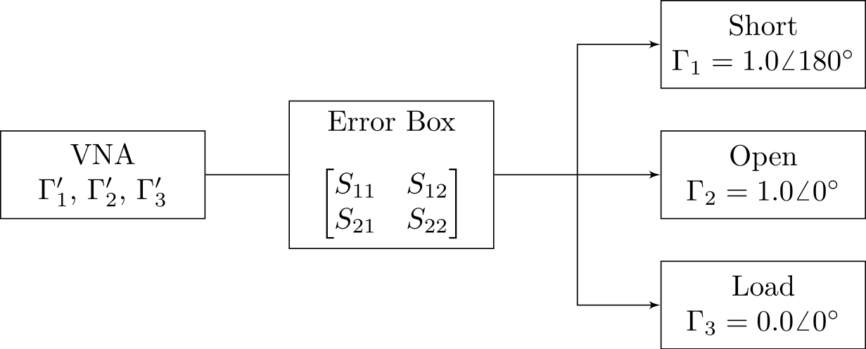
Single-port calibration is the foundation of multi-port calibration. For single-port measurements, the most common VNA calibration method is Short-Open-Load (SOL) calibration. By measuring an ideal short (reflection coefficient Γ1=1.0∠180∘), an ideal open (Γ2=1.0∠0∘), and an ideal load (terminating resistor, Γ3=0), and comparing these with the VNA’s own readings Γ1′,Γ2′,Γ3′, the SOL algorithm can solve the signal path’s own contribution and remove it from future measurements.
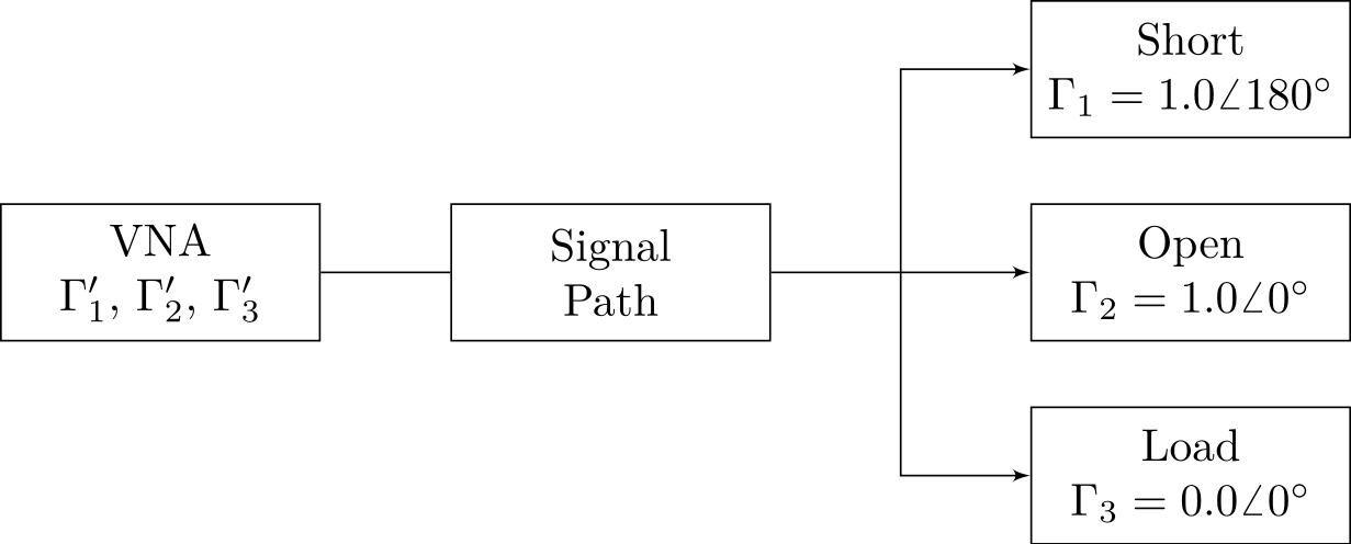 Calibrating the VNA eliminates the
effects of the signal path
Calibrating the VNA eliminates the
effects of the signal path
Parasitic Parameters of Calibration Standards
In practical circuits, parasitics are ubiquitous. An open-ended transmission line has a small parasitic capacitance at its end, as part of the electric field exists in the air around the cable; a shorted transmission line also has a small parasitic inductance at its end. If the calibration standard’s body is not precisely located at the connector interface but slightly away from it, it introduces a small section of offset transmission line, creating additional phase deviations.
Therefore, perfect open and short standards are unattainable; their reflection coefficients cannot remain constant at 0∘ or 180∘ but must vary with frequency.
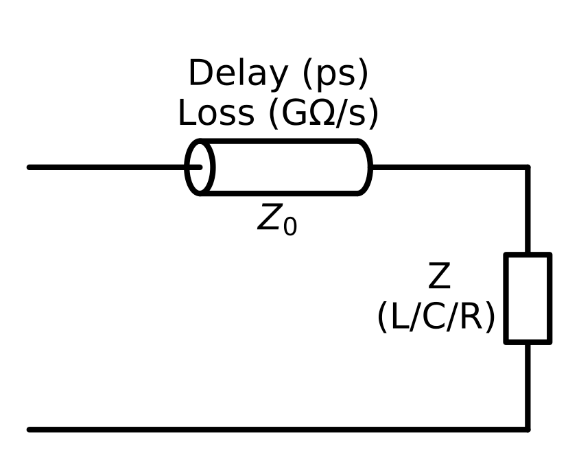 Equivalent circuit model of calibration
standards
Equivalent circuit model of calibration
standards
The purpose of creating a set of calkit is not to create perfect devices “without parasitics” but to create practical devices with stable, known parasitics. During VNA calibration, the errors are the unknowns in the equations, and the imperfect calkits themselves are the known coefficients. They can take any value, not necessarily 0 or 180 degrees. When solving the equations, the calkit’s own errors are already excluded, and the true error of the signal path is calculated. Clearly any device can be used as standards in principle - as long as its electrical characteristics are known and repeatable, even if it has a crude appearance and has significant “parasitics.” Calibration error is not determined by “parasitics” but by the accurary of their definitions.
Generic Calkits
Stock calkits from VNA vendors are backed by the original manufacturer’s reputation and decades of use, offering stable performance, but with a high price tag. Even second-hand products can cost nearly $1000-$2000. On the other hand, there are many simple, generic calkits on the market, selling for as little as $5 on Taobao, eBay, or AliExpress — no manufacturer, no model number, no definitions, primarily serving amateur radio applications. Since they lack characterization, their accuracy is unknown, so we naturally ask: Can these calkits be used for everyday measurements with modest requirements? How large will the measurement error be?
A vendor attempted to answer this question for readers in an article published on the company’s official account, titled How Large is the Phase Error of Commercially Available VNA Open and Short Calibration Kit? [1]. In the article, the vendor claimed to use an Agilent E5071C VNA and, using Agilent 85033E and 85032F calkits as references, measured the electrical characteristics of generic SMA and Type-N standards, reaching this conclusion:
So, how big is the impact? You wouldn’t know without looking, and it’s startling to see… The phase deviation of open and short standards from VNA calibration kits without extracted parameters isn’t a simple 5 or 10 degrees. It’s errors of tens, even hundreds of degrees.
The vendor told readers that the simple, generic calkits on the market have huge errors. In contrast, readers should purchase characterized calkits. Coincidentally, exactly what this vendor is selling: Low-cost calkits. Unlike other cheap products, their products are slightly higher-end. Although inexpensive, they have characterized electrical delays.
Certainly, characterized calkits are superior to generic, unknown calkits. As part of a personal project, the author has tested many inexpensive calkits, including those from this vendor. This data has not yet been carefully analyzed (to be published later), but preliminary results already show that the vendor’s calkits are reasonably accurate and fully meet daily application needs. We do not deny the usefulness or quality of the vendor’s calkits.
However, did the vendor’s article clearly and fairly present the true electrical characteristics of the generic calkits to readers? We can easily identify some obvious problems.
Problems
Issue 1: Physics-Defying Counter-Clockwise Phase
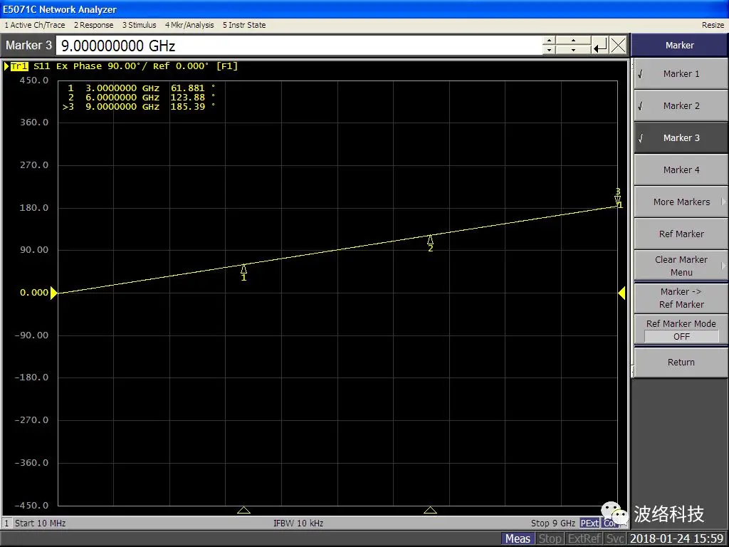
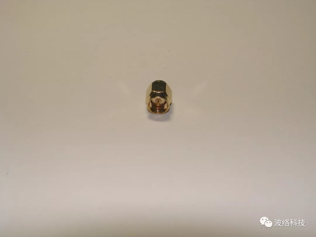
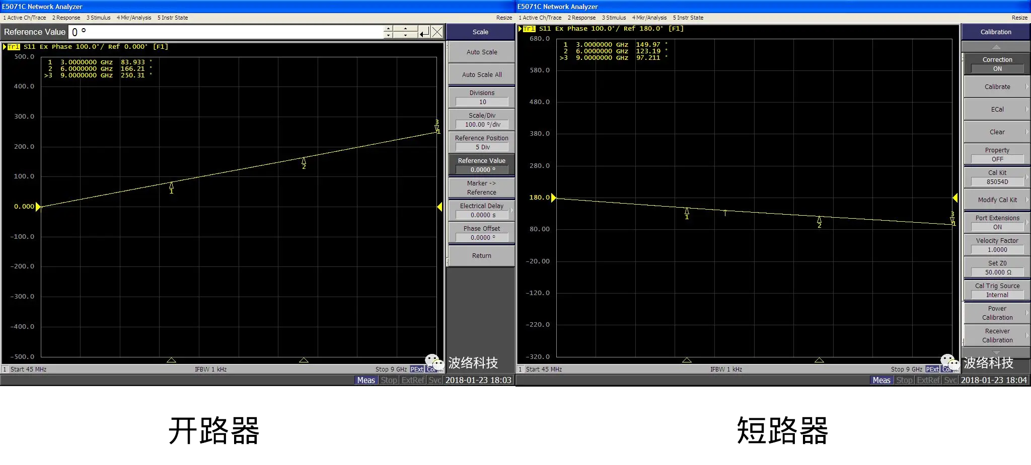
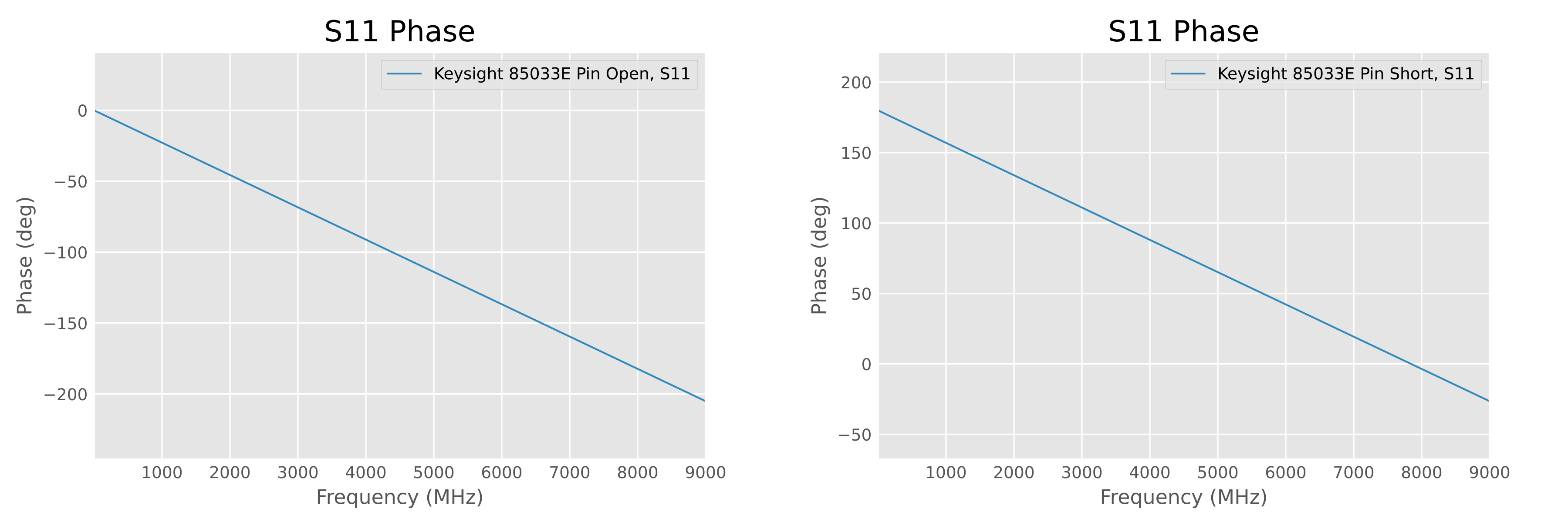
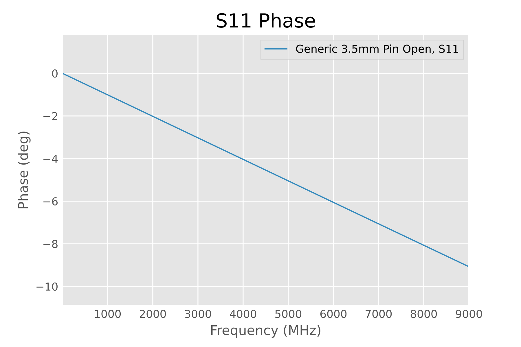
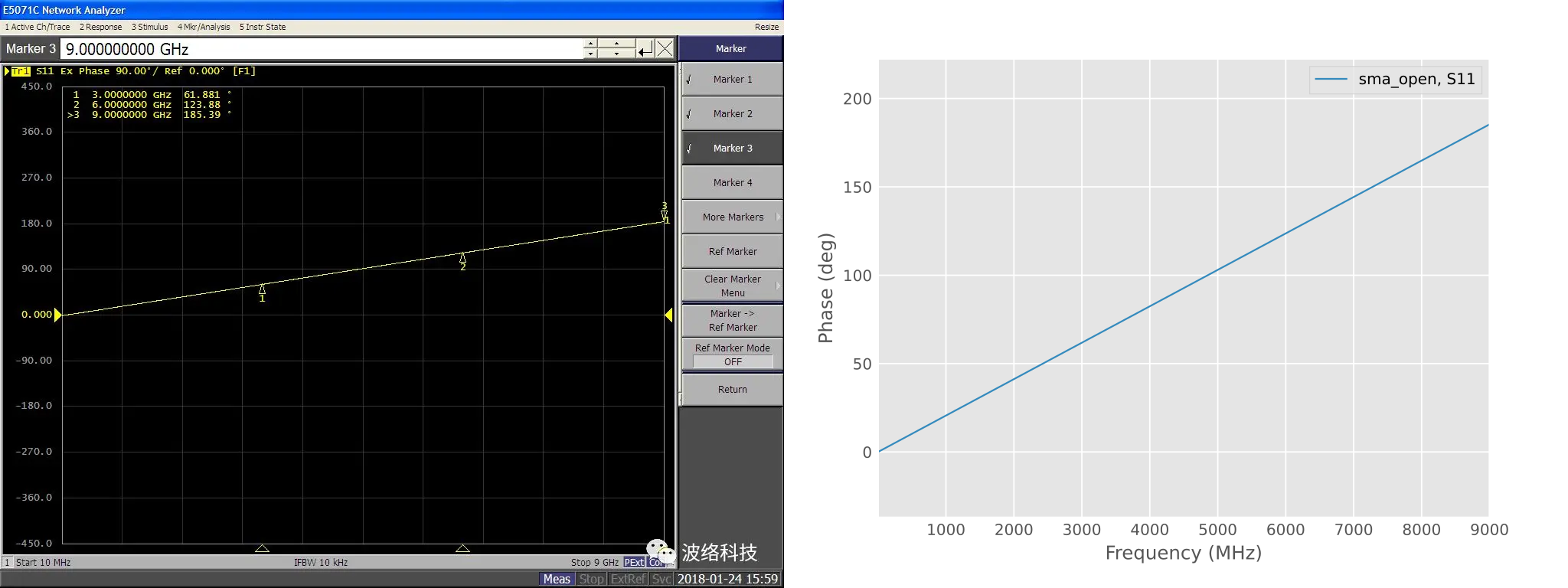
The vendor measured the phase response of generic SMA open and short standards.
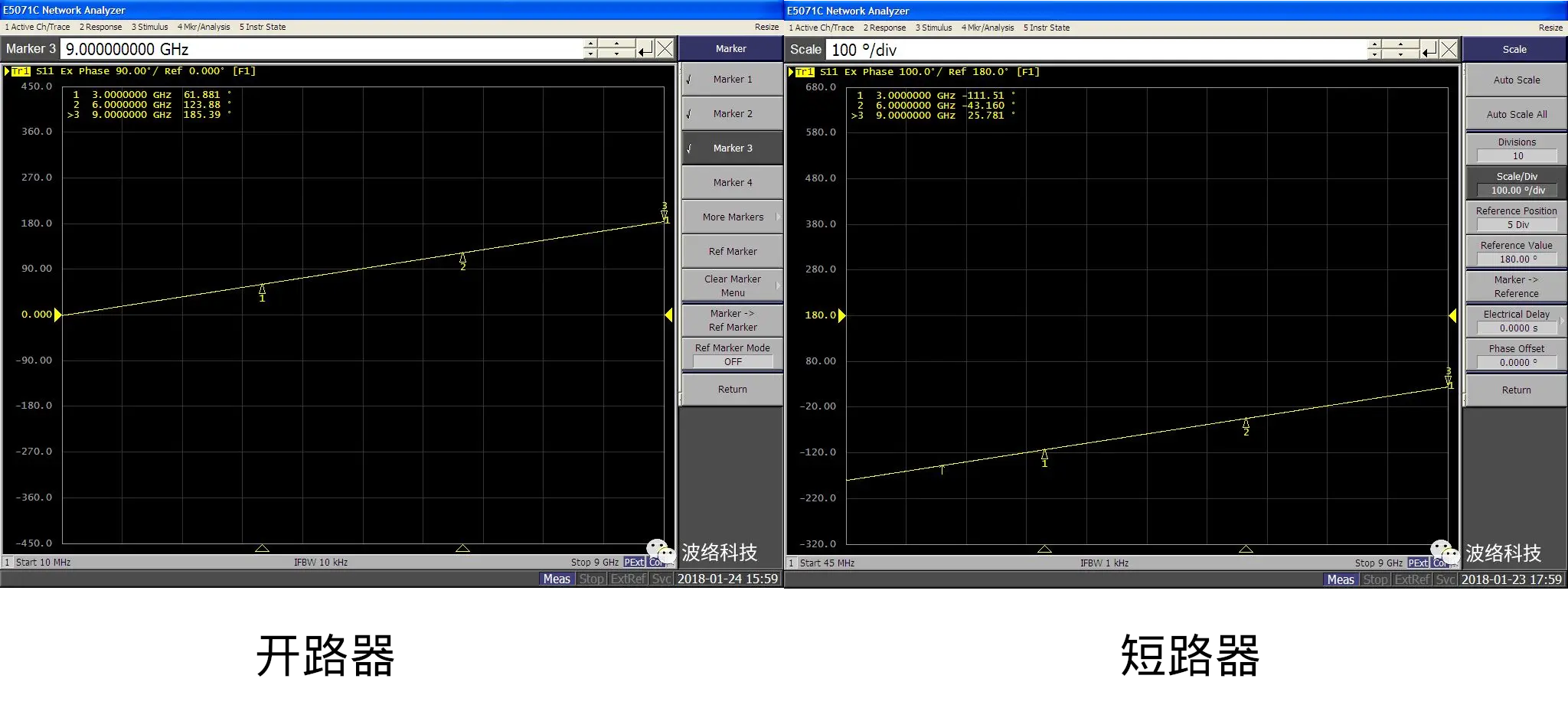 Measurement of generic Open and Short
standard published by the vendor.
Measurement of generic Open and Short
standard published by the vendor.
Let’s observe these two graphs: as the frequency increases from 0 GHz to 9 GHz, the phase of both devices consistently moves in the positive direction. Even ignoring their numerical values, the sign alone is a literal sign of trouble.
What does this mean? If one just looks at the line charts, it might not be obvious, but if the data is plotted using polar coordinates, this means the phase has a counter-clockwise (CCW) rotation on the Smith chart. Any lab worker with common sense would recognize anomalous data: any passive RF device made from “ordinary” materials found in nature should have an overall clockwise phase rotation, not a CCW rotation. Negative phase represents phase lag, positive phase represents phase lead. CCW phase rotation violates common-sense physics; it implies negative capacitance, negative inductance, or negative transmission line delay. The signal was received before it was transmitted? Was this network analyzer measuring a microwave signal or a “PhoneWave” signal?
Of course, “CCW phase” can indeed be achieved in the laboratory using resonant circuits, metamaterials, or active devices: “left-handed transmission lines” are a classic case. In “fast light” materials, group velocity can even exceed the speed of light. But these metamaterials only work in narrow frequency bands, not across the full 0-9 GHz range. Anyone discovering such a metamaterial would absolutely deserve an IEEE Fellowship. But simple $5 SMA connectors on eBay would never be the birthplace of this groundbreaking discovery.
According to industrial engineering standards, such data should not be analyzed further but discarded as invalid. As the IEEE P370 standard [4] states:
Initial causality estimation is performed in the frequency domain, and is based on the observation that a polar plot of a causal interconnect rotates mostly clockwise (first suggested by V. Dmitriev-Zdorov and described in Shlepnev). […] To evaluate the “amount” of the clockwise versus counterclockwise rotations, a preliminary causality quality metric (CQMi) can be introduced as follows […]
- (80, 100] — Good
- (50, 80] — Acceptable
- (20, 50] — Inconclusive
- [0, 20] — Poor
What score does the vendor’s data get? 0.
Issue 2: Open Phase Shift Exceeds Literature Values by 10x
Beyond the sign problem, let’s look at the numerical values. The vendor “discovered” that the open standard’s phase soared from 0 degrees at 0 GHz to a startling 185.39 degrees at 9 GHz.
 Open standard values
Simultaneously, the vendor described the construction of the measured open standard in the article:
This is the construction of the vast majority of commercially available mid-to-low-end open standards; it’s simply an empty cavity in the middle. Perhaps some manufacturers lengthen the housing to make it look more premium. The actual electrical performance is the same.
 Open standard construction
However, the vendor seems completely unaware of the contradiction between their statement and their data. We must be clear: the typical parasitic value of a coaxial open circuit is not some unsolved mystery but a classic problem studied since World War II. Lengthening the housing is not merely for show but to satisfy electromagnetic theory.
The theoretical basis for the open standard is “the transition of a coaxial transmission line to a circular waveguide below cutoff frequency,” a classic electromagnetics problem. The most ingenious aspect of this open standard is that it utilizes the physical phenomenon where “electromagnetic waves do not propagate in a circular waveguide below cutoff but become rapidly decaying evanescent waves.” It creates a physical structure with a well-defined capacitance, overcoming the uncertainty of electromagnetic radiation and the influence of surrounding objects. Thus, it was once a type of metrology standard—lengthening the housing is meant to bring it closer to the “infinite length circular waveguide” condition. Although the practical difference is likely negligible for SMA connectors, doing so is a form of “electromagnetics puritanism.”
![Coaxial transition to circular waveguide below cutoff[5]](https://niconiconi.neocities.org/img/review-of-a-misleading-vendor-article-on-vna-calibration/chramiec-and-piotrowski-geometry.png) Coaxial transition to circular waveguide
below cutoff[5]
Coaxial transition to circular waveguide
below cutoff[5]
As early as 1944, J. R. Whinnery’s papers [6], [7] preliminarily studied the equivalent circuits of transmission line discontinuities; similar formulas were also recorded in Volume 10: Waveguide Handbook (1951) [8] of the MIT Rad Lab Series—a summary of MIT’s wartime research; in the 1960s, P. I. Somlo used a mainframe computer to calculate it to five significant digits [9], [10], far exceeding experimental accuracy, almost closing the issue. Subsequent recalculations using other methods showed only minor differences (e.g., [11], [12]), and lacked detailed design charts, so Somlo’s papers remain the standard reference. Because coaxial probes can be used for permittivity measurement, needs in materials science and biology also drove further research on this problem; Finite Element Method (FEM) and Method of Moments (MoM) were also used for calculation in the 1980s [13]; in 2023, the UK’s National Physical Laboratory (NPL) used this problem to compare the accuracy of different solvers [14] (one of the authors, Hodgetts, was himself a 1980s veteran researcher on the same issue [15]).
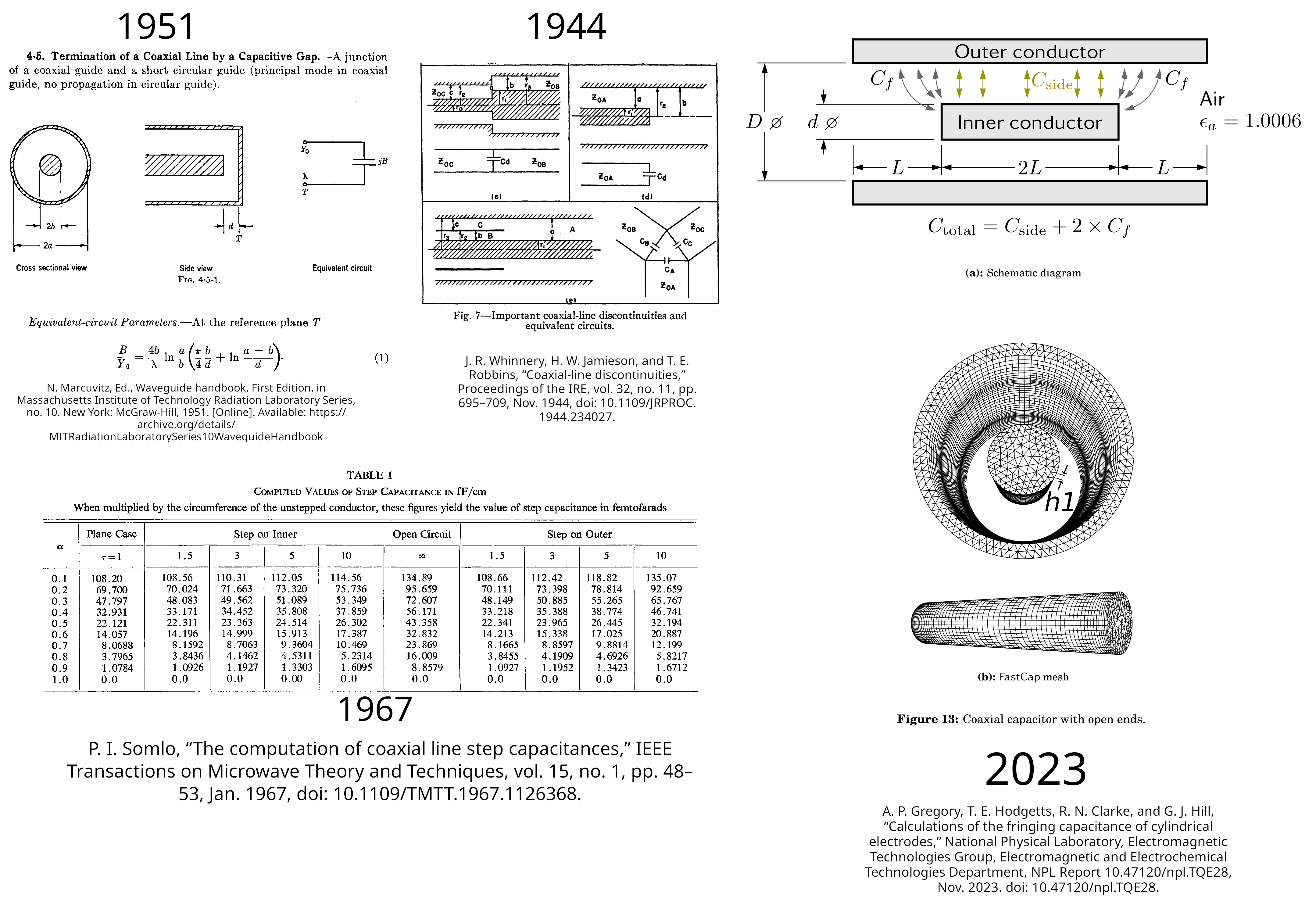 Coaxial transmission line open-end
capacitance has been researched for 80 years
Coaxial transmission line open-end
capacitance has been researched for 80 years
For a Z0 = 50 Ω, 3.5 mm air transmission line, the accepted result is: the equivalent capacitance at the end should be 30-40 fF (0.03-0.04 pF), see Appendix 4: Calculation of Open-Ended Coaxial Line Fringe Capacitance. Real SMA connectors are not ideal coaxial lines, so deviations are to be expected (the author’s preliminary experimental data shows many influencing factors). But claiming the open standard has phase errors of “tens, even hundreds of degrees” is utterly unreasonable.
We know the relationship between an ideal capacitor and reflection phase is:
Zcap=−j12πfCarg(Γcap)=arg(Zcap−Z0Zcap+Z0)
At 9 GHz, a 40 fF parasitic capacitance equates to a 12.9 degree phase shift, while a 100-degree phase shift equates to a 421 fF capacitance. If the “100-degree error” were true, it would mean exceeding the accepted value by over 1000%, completely overturning 80 years of scientific consensus—does electromagnetics no longer exist? The vendor is possibly a Trisolaran agent sent to hinder Earth’s science.
Issue 3: Short Phase Shift Exceeds Normal Value by 40x
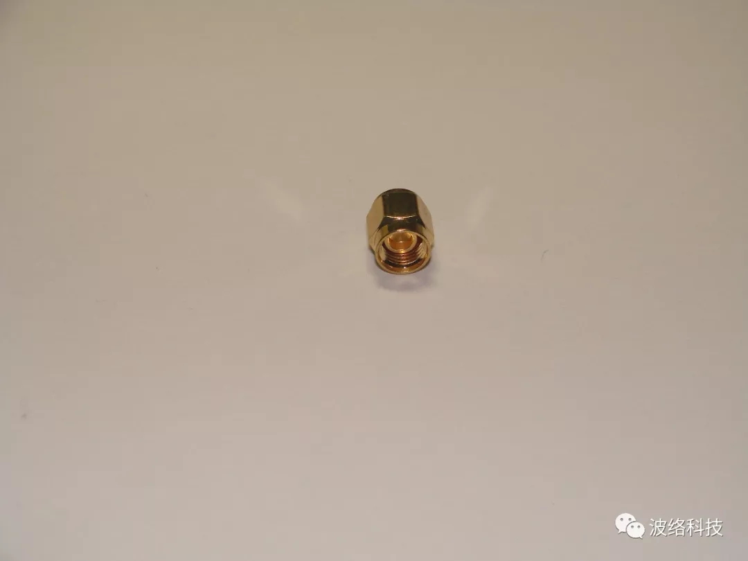
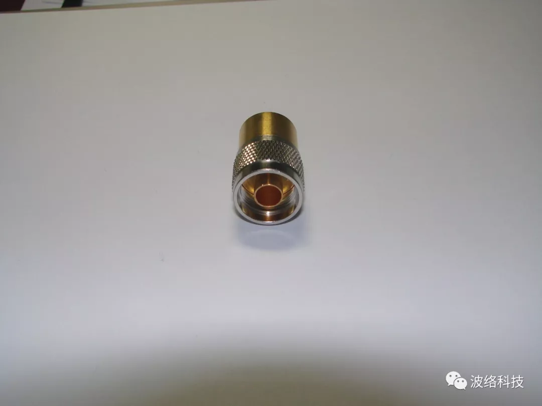
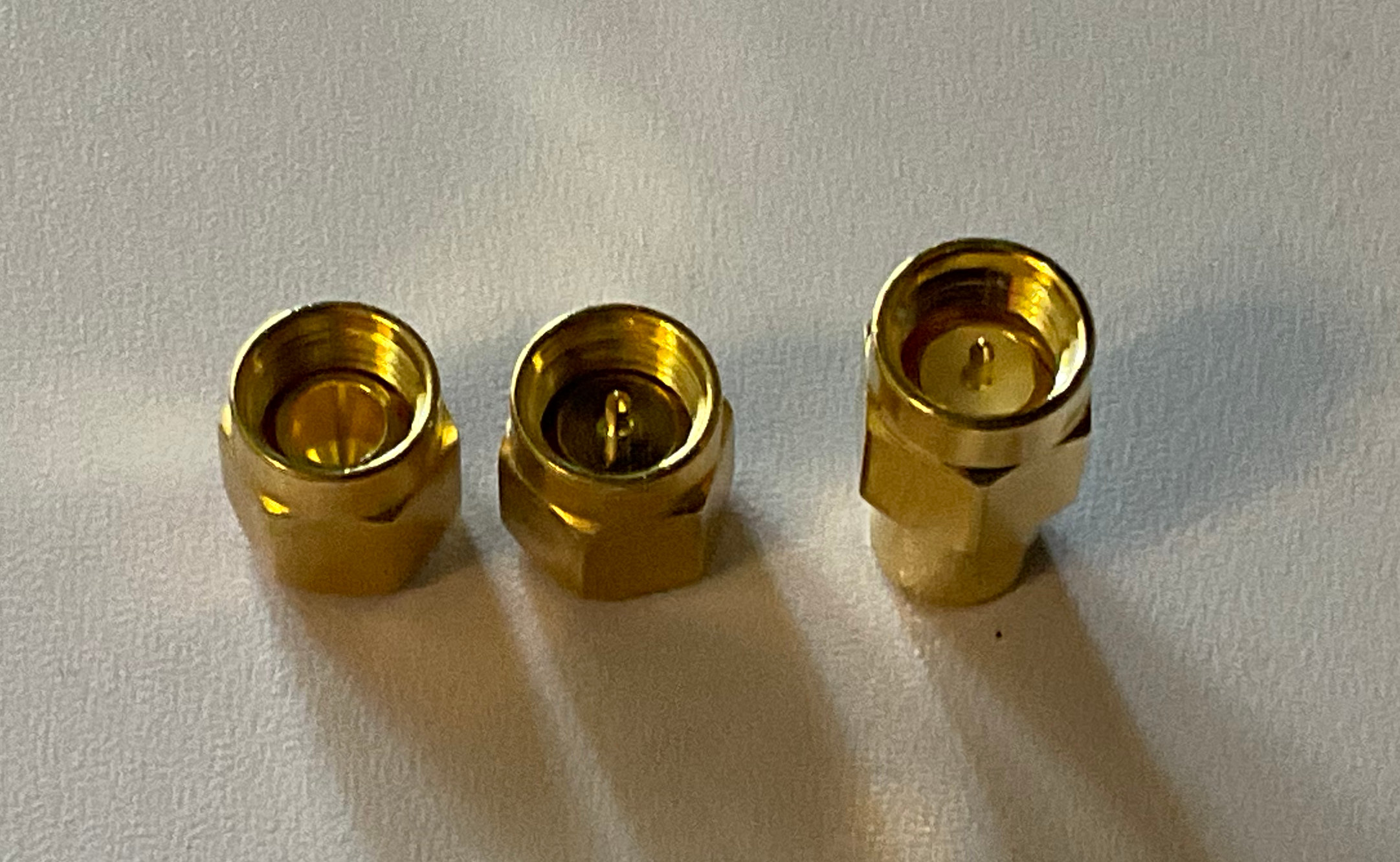
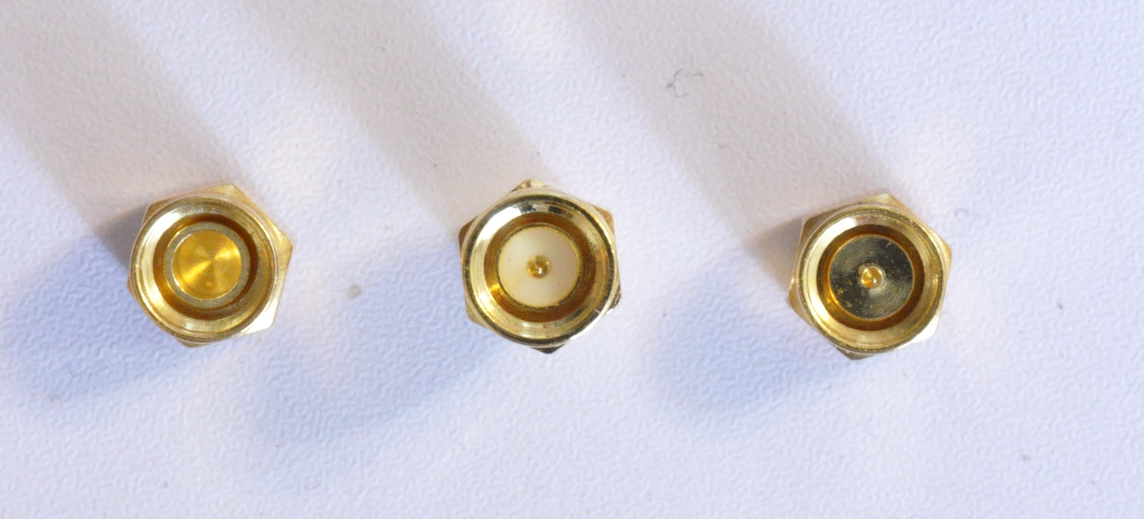
The short standard has a similar problem. The vendor showed readers a photo of the measured generic short standard, showing it is a simple SMA plug. The end of the center pin, no longer having an insulator, is directly connected to the metal shell, creating a short circuit.
 Short standard construction
The vendor claimed this extremely simple short standard produces a total phase shift of 205 degrees, which is alarming. However, this also blatantly contradicts how SMA/3.5 mm connectors work.
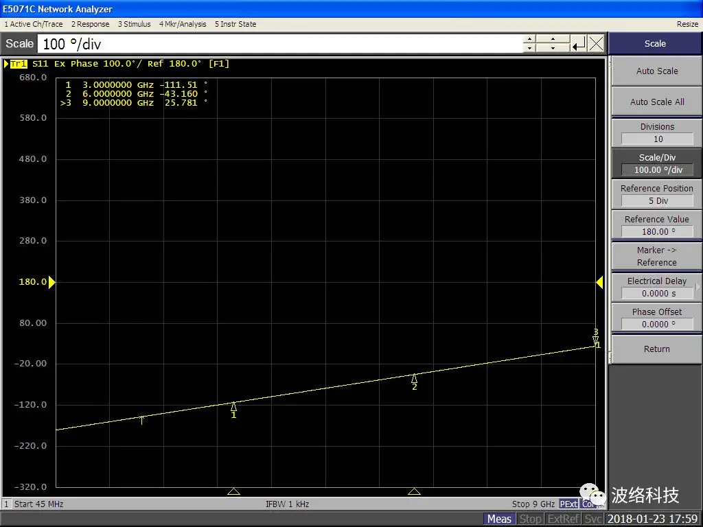 Short standard values
We need to know: the core design philosophy of SMA/3.5 mm is “well-defined reference plane.” In microwave measurements, any cable length introduces delay and phase shift, so all measurements must define “where is the point being measured?” This point is called the measurement’s “reference plane.” VNA calibration essentially re-establishes this reference plane, moving it to the end of the last connector of the last cable. Because the connector itself has length, precise measurement is impossible if its internal reference plane is unclear. Connectors originating from the 1940s, like the Type-N (and its derivative BNC), have this problem: the inner and outer conductors meet at different points, making the reference plane unclear [16]. Type-N connectors are still used only because of extensive error analysis work.
Connectors from the 1960s onwards, like SMA/3.5 mm, follow a new principle: the reference planes of the plug and socket are clearly defined and coincident, i.e., the plane indicated by “Note 1” in the figure below.
![International standard drawing of SMA connector interface[17]](https://niconiconi.neocities.org/img/review-of-a-misleading-vendor-article-on-vna-calibration/iec61169-15.png) International standard drawing of SMA
connector interface[17]
International standard drawing of SMA
connector interface[17]
We can see an SMA connector consists of two parts: the connection part (hole and pin) and the body transitioning to the cable. The connection part has strict technical requirements: for a socket, its outer conductor and inner hole reference plane align and are located at the start of the hole (the position of the SMA insulator); for a plug, its outer conductor and center pin reference plane also align, both located at the bottom of the plug’s center pin (again, the position of the SMA insulator). When the plug and socket are connected, the outer conductors, center pins, and insulators of both connectors all meet at the same point. A destructive teardown by @TubeTimeUS [18] nicely demonstrates this ingenious design: the two connectors are almost seamless—the end of one cable is precisely the beginning of another. This minimizes air gaps and avoids impedance discontinuities.
![Destructive teardown by TubeTimeUS[18]](https://niconiconi.neocities.org/img/review-of-a-misleading-vendor-article-on-vna-calibration/mated-sma.png) Destructive teardown by TubeTimeUS[18]
Destructive teardown by TubeTimeUS[18]
For a generic SMA short standard with no cable body, no extra structure, and a complete short circuit, it is essentially a pure plug. According to the international standard IEC 61169-15, the gap between plug and socket is not allowed to exceed 0.25 mm [17]. Therefore, the generic short standard is almost a flush (zero-length) short. When fully inserted into an SMA/3.5 mm socket, its reference plane falls exactly at the position of the shorting outer shell (the original insulator position).
Literature shows that a metal shorting plate at the end of a coaxial transmission line has a phase shift of only about 0.1 degrees even at 110 GHz [19], [20], [21]. This indicates that the short standard’s error does not come from the short itself but mainly from the connector body’s length and tolerances, equivalent to extending the transmission line. Since the generic flush short has virtually no internal extension, the only source of error is the air gap created by tolerances.
In air, the relationship between the physical length of an ideal transmission line and the reflection phase is:
arg(Γline)=2⋅(−360∘⋅flc)⏟One-way phase shift
Calculations show that a 0.25 mm transmission line produces about 5 degrees of worse-case phase shift (at 9 GHz); however, the vendor’s “205-degree phase shift” is equivalent to 9.5 mm of air transmission line—why does the careful design of SMA/3.5 mm result in an error magnified by 40 times in the vendor’s hands?
Issue 4: Suddenly “Normal” Type-N Short Data
Among the four measurement screenshots, the vendor’s “Type-N short” screenshot exhibits other conspicuous anomalies.
 Generic Type-N open standard as measured
by the vendor
Generic Type-N open standard as measured
by the vendor
 In the vendor’s screenshot, the short
standard’s phase suddenly returns to normal
In the vendor’s screenshot, the short
standard’s phase suddenly returns to normal
Upon closer inspection, the other three measurement results show anomalous positive phase shifts, but only when measuring the Type-N short, the VNA suddenly “returns to normal,” displaying a seemingly “reasonable” negative phase shift.
Only in this screenshot does the “Calibration” menu appear on the right side of the screen. However, according to the timestamps on the four screenshots, the vendor measured the generic SMA short at 2018-01-23 17:59, the Type-N open at 18:03, the Type-N short at 18:04, and finally the SMA open the next day at 15:59. The Type-N short was the last device measured that day. Typically, calibrating the VNA is preparation done before starting measurements. Why did the vendor suddenly enter the calibration menu just as the measurements were concluding? Perhaps it was a misclick, but coincidentally the VNA data just happens to return to “normal,” raising questions.
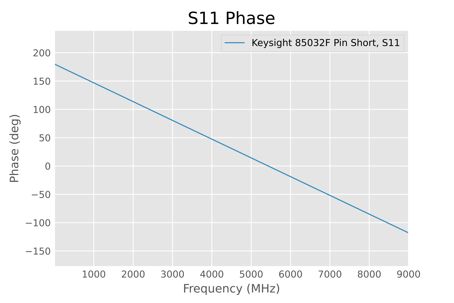
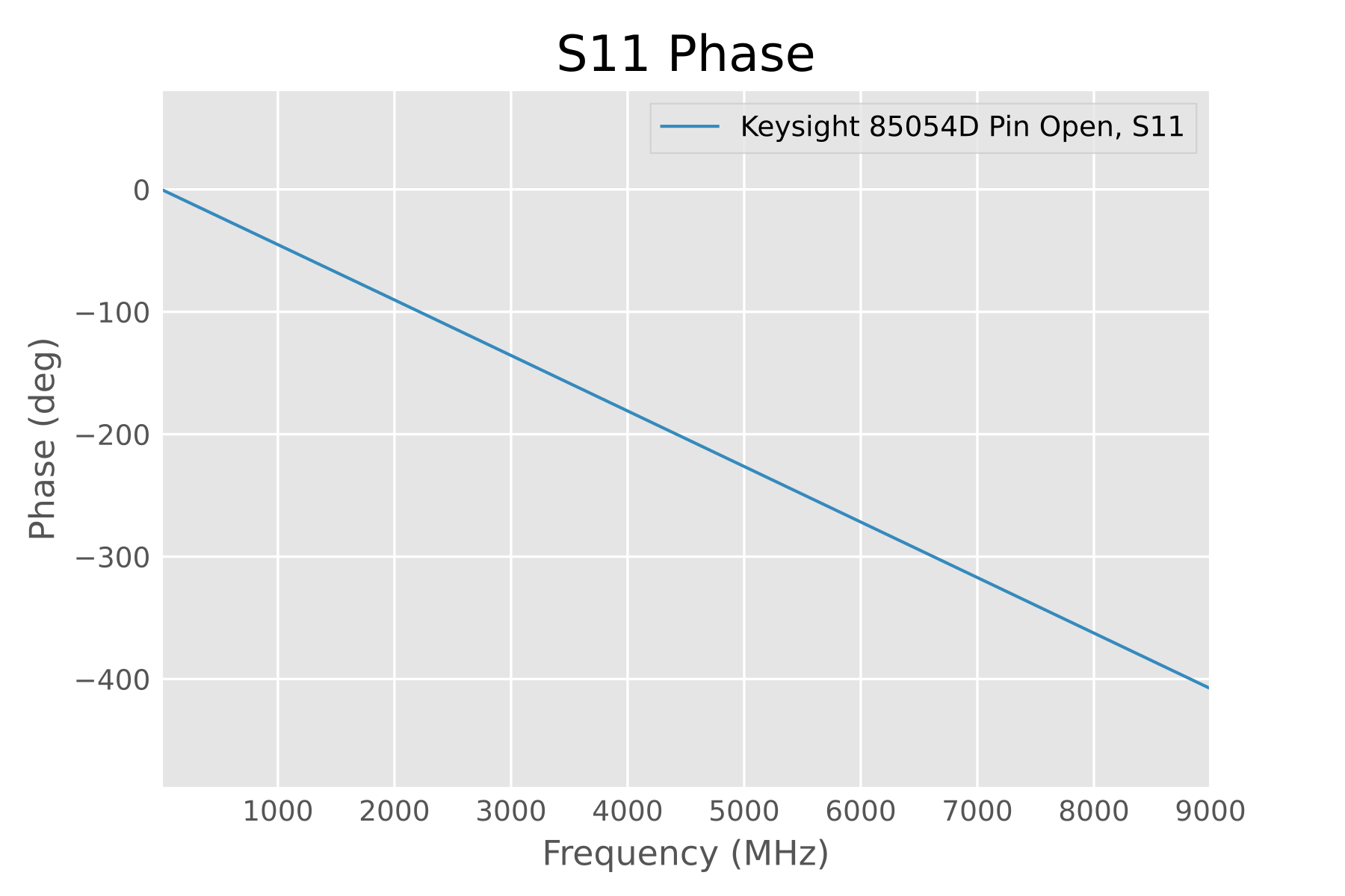
Even stranger, the vendor explicitly stated at the beginning of the article that they “used Agilent’s 85032F as a reference,” but the screen shows “Correction: ON”, “Calkit: 85054D”. The highlighted “Correction: ON” button further suggests this was the vendor’s last operation.
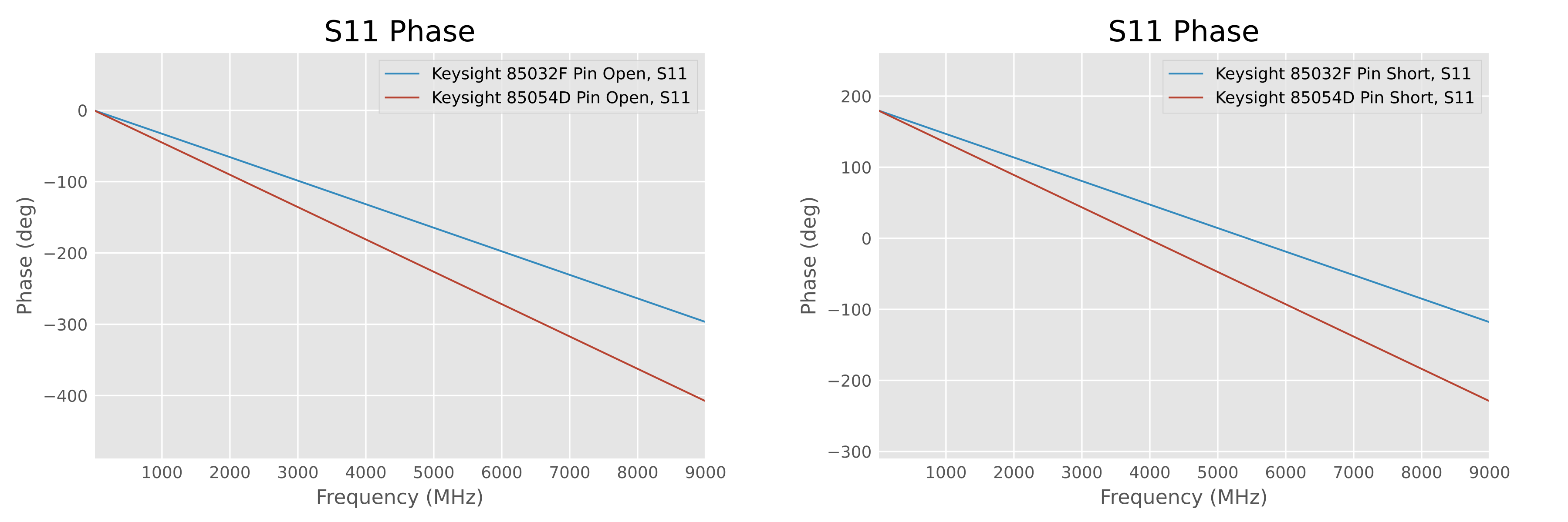
According to the stock calkit definitions published by Keysight [22] (see Appendix 3: Equivalent Circuits of Calibration Standards), the electrical characteristics compare as follows:
 Phase response comparison of Agilent
85032F and 85054D
Phase response comparison of Agilent
85032F and 85054D
These are two calkits with noticeably different phase shifts. So why did the vendor claim to use “85032F” but have “85054D” enabled at this time?
Data Mystery
Considering the above points, we can only conclude that the measurement data presented on the screen is utterly wrong due to erroneous operation; or it is technically correct but presented in a severely misleading way. Under what circumstances would the instrument display such absurd phase values?
Phase Difference Hypothesis
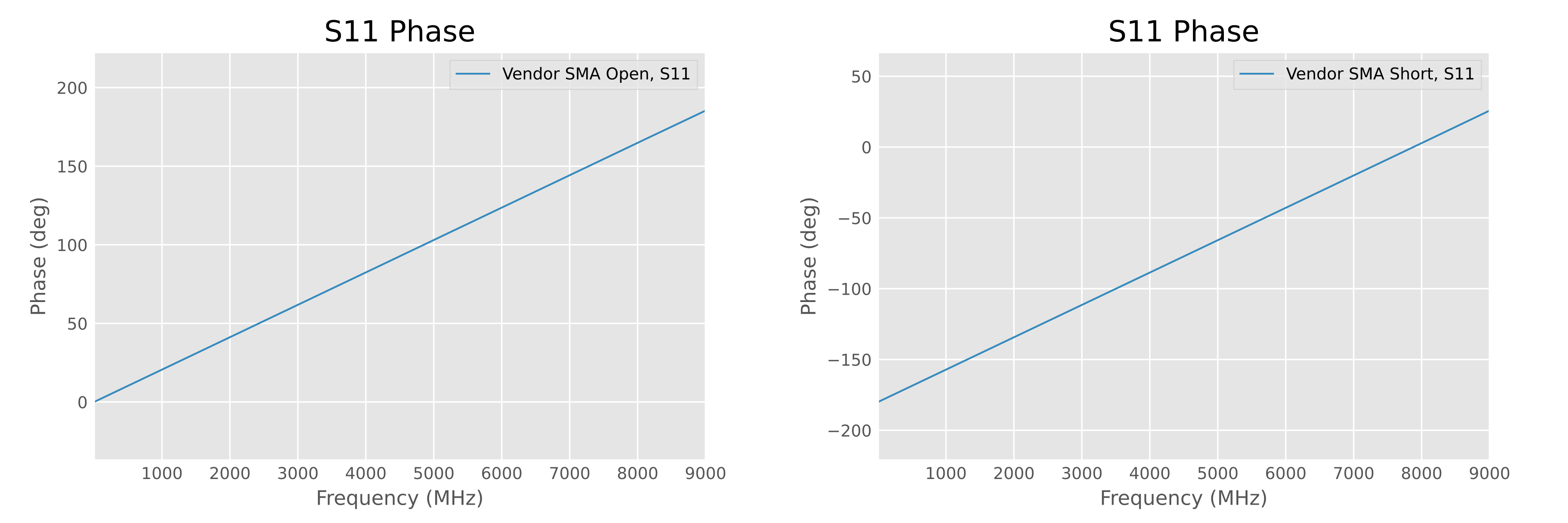
To investigate this issue, we reverse-engineered the raw measurement data of the open and short standards claimed to show “huge errors” from the vendor’s screenshots. Credit is due to the vendor for thoughtfully providing three markers, with phase values at three frequency points accurate to three decimal places, which undoubtedly greatly aided our extraction work. Using linear interpolation, the original data can be accurately recovered; see Appendix 2: Reverse Engineering Vendor Data for the specific method.
 Reverse-engineered raw data (see appendix
for method)
Reverse-engineered raw data (see appendix
for method)
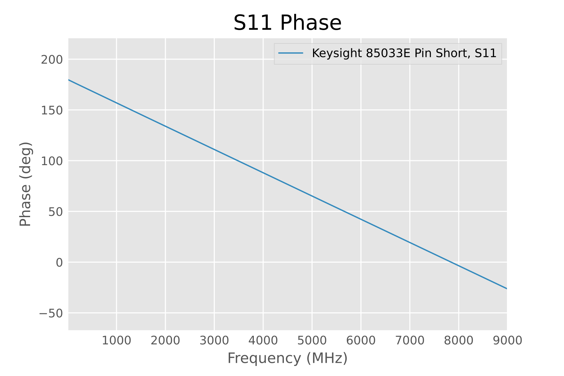
The definition data for the stock standards is publicly available from Keysight [22]. Since the vendor said they used “Agilent 85033E”, we reproduced the stock data for comparison (see Appendix 3: Equivalent Circuits of Calibration Standards for the method):
 Independently reproduced phase response
of Agilent 85033E calkit (see appendix for method)
Independently reproduced phase response
of Agilent 85033E calkit (see appendix for method)
We were surprised to find that these two graphs seem to be symmetric about the X-axis! What happens if we flip the sign of the vendor’s so-called “huge error” measurement data?
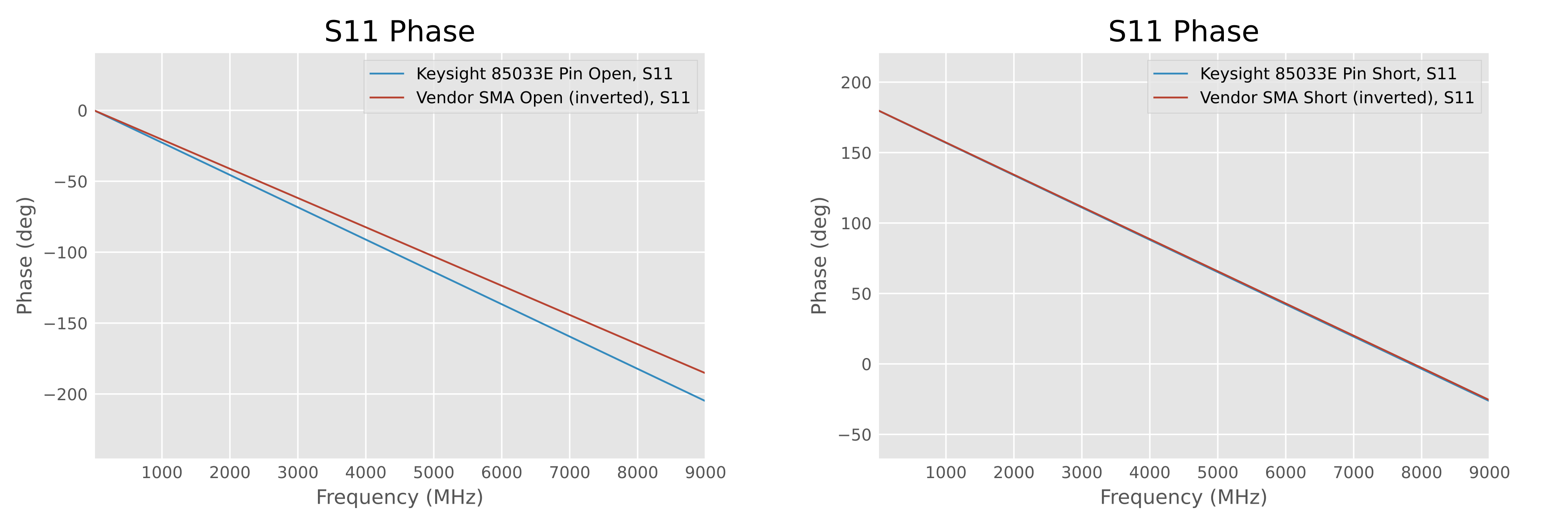 Compare the vendor’s data (sign inverted)
with Agilent 85033E
Compare the vendor’s data (sign inverted)
with Agilent 85033E
We can see that the sign-inverted phase becomes a normal clockwise phase shift and closely resembles the phase of the Agilent 85033E, with the short standard almost perfectly overlapping!
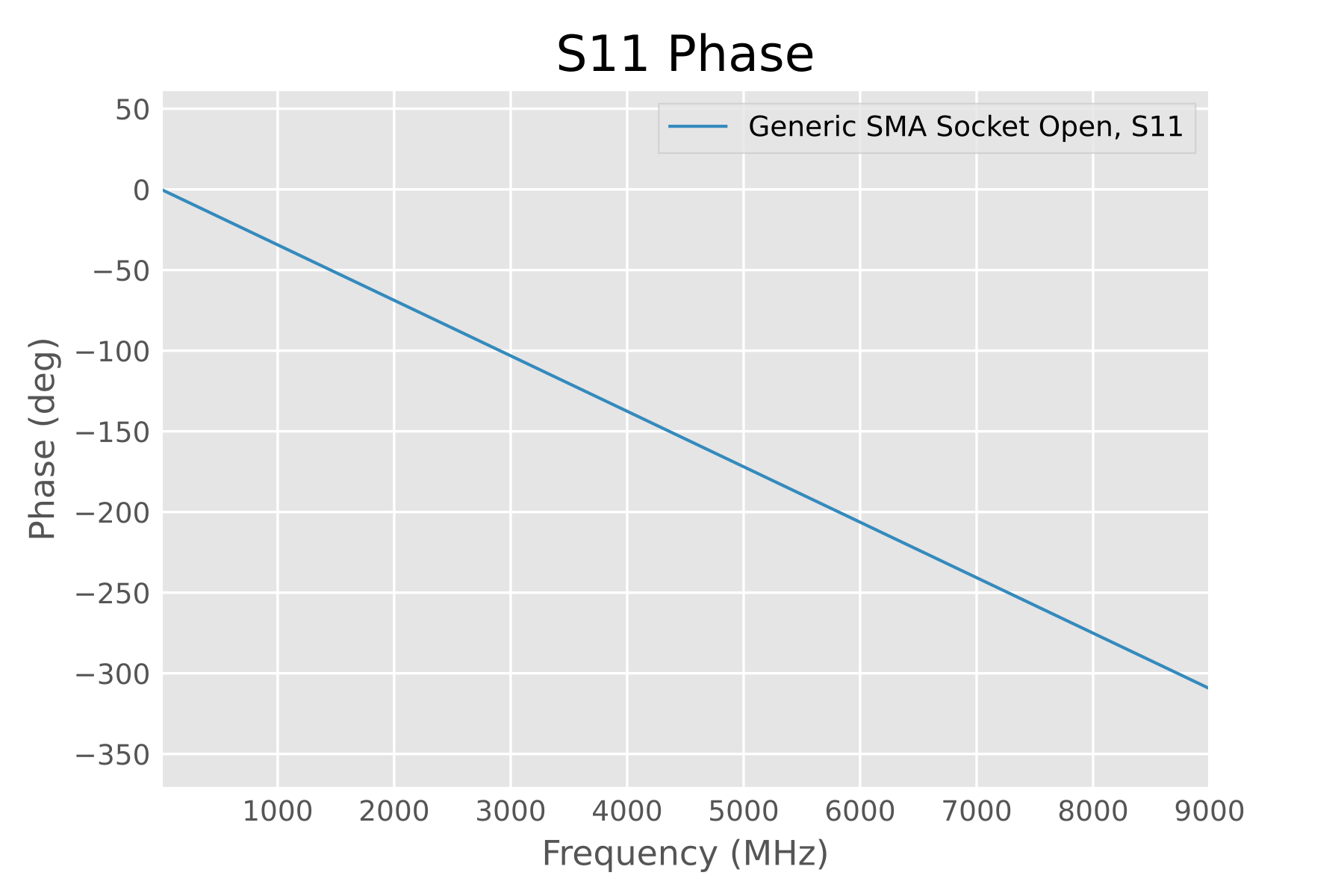
This inevitably leads to the suspicion that the vendor used a relative measurement mode: the vendor measured not the phase response of the generic calibration standard itself, but the phase difference between the generic calkit and the stock calkit. In fact, they belong to two distinct types of coaxial calibration standards: “zero-length” standards and “offset” standards.
 “Flush” standards sit flush against the
connector, with no additional extended structure
“Flush” standards sit flush against the
connector, with no additional extended structure
Due to good repeatability, most stock calkits are offset standards. Unlike flush types, offset standards have a small section of transmission line in front, acting as a delay line, inherently introducing a large negative phase shift. Flush standards only have the small phase shift introduced by parasitics.
 “Offset” standards have an extended body,
introducing additional delay
“Offset” standards have an extended body,
introducing additional delay
Taking the open standard as an example, subtracting a larger negative number (stock open phase) from a smaller negative number (generic open phase) results in a positive number:
ϕreading=ϕgeneric open−ϕstock open≈0∘−(negative number)=positive number
The vendor might not want readers to obtain the true frequency response of the generic standards—if readers had the data, they could characterize their own generic standards, rendering the vendor’s characterized products less meaningful. Presenting the data in this highly misleading way could conceal the raw data. If we want the true open standard phase shift, we can try subtracting the stock phase from the measurement result—this shows the true generic open standard’s phase leads the stock standard by 0-20 degrees (at 9 GHz), while the short standard has almost no phase difference. This result is entirely reasonable.
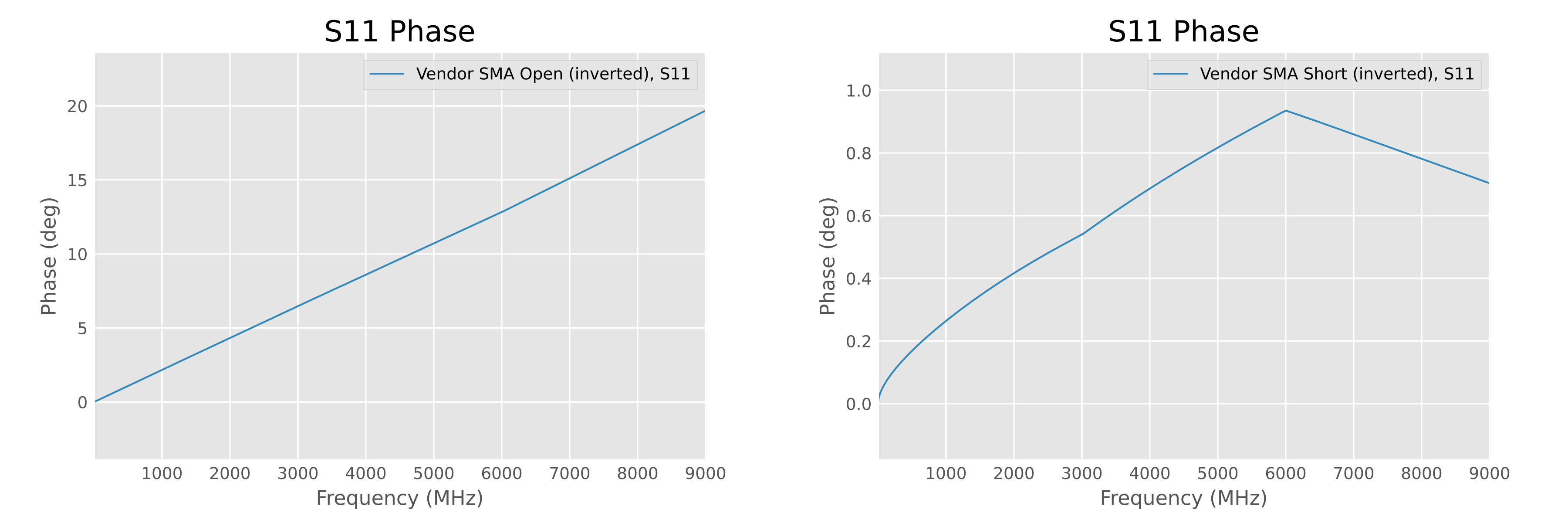 Relative phase shift between vendor’s
measurement result (sign inverted) and Agilent 85033E
Relative phase shift between vendor’s
measurement result (sign inverted) and Agilent 85033E
But this “phase difference hypothesis” is not without flaws. In the raw data for the generic short, its phase difference is -180 degrees at 0 GHz. However, at low frequencies, both generic and stock shorts should have the same -180 degree phase shift, making the relative phase difference 0 degrees (not 180 degrees). Furthermore, there seems to be no indication on the VNA screen that the relative measurement function was enabled, suggesting the screen displays “absolute” phase (phase relative to the incident wave, not relative to another standard)—this completely overturns our hypothesis.
Zero-Parameter Calibration Hypothesis
What method could make a VNA interpret a negative phase shift as positive? Through repeated experimentation, the author found a method that can reproduce similar measurement data: zero-parameter calibration.
First, we recalibrate the VNA. During calibration, we use the stock Agilent 85033E calkit but enter “all-zero” definition parameters into the VNA. That is, even though the open and short standards have negative phase shifts, we tell the VNA that these standards are “ideal with no phase shift.” After calibration, the VNA’s phase zero point shifts in the negative direction. Thereafter, any device with an absolute phase deviation smaller (more positive) than the Agilent standards will have falsely larger values. The higher the frequency, the greater the inherent phase shift of the stock standards, the further the zero point shifts negatively, and the more the measurement data is exaggerated in the positive direction. This causes the phase of the generic short to move positively, even becoming positive.
ϕhigh freq reading=ϕgeneric short−ϕzero point≈−180∘−(negative number)=positive number
Simultaneously, since only at high frequencies do the standards have significant phase shifts. At low frequencies, the true zero point is unaffected, so the correct “absolute” phase will still be correctly displayed on the screen—thus, the short’s phase shift at 0 GHz remains -180 degrees, unlike the 0 degrees displayed in relative measurement.
ϕlow freq reading=ϕgeneric short−ϕzero point≈−180∘−0∘=−180∘
The figure below shows the erroneous measurement results simulated using scikit-rf. We first initialize the SOL calibration algorithm using the stock Agilent 85033E but mistakenly use all-zero parameters. We then measure an open and short standard with tiny parasitics. The open and short measurement results both shift positively (red curves), reproducing data similar to the vendor’s “counter-clockwise phase.” The algorithm was told the 85033E has no parasitic parameters or phase error, so the standards’ phase shifts are converted into instrument zero-point drift (blue curve).
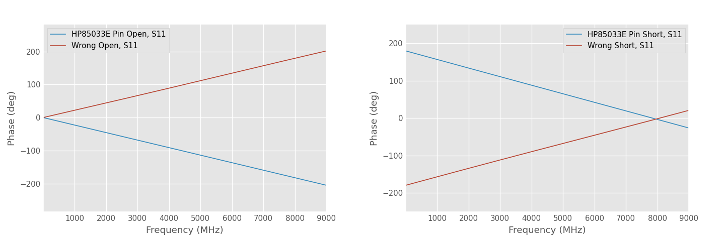 Simulation of miscalibration
effect
Simulation of miscalibration
effect
A similar operation might have been performed for the Type-N short. Perhaps the “error deviation” measured using the “miscalibration method” was too small to achieve a startling dramatic effect. Therefore, the vendor might have switched the calibration to the doubly erroneous 85054D definition —pretending they have measured a “huge error.”
Reproducing the Mis-calibration
We can independently reproduce this mis-calibration using simple Python code and numerical methods. The algorithm workflow is as follows:
- Calibrate a virtual VNA using virtual Agilent standards, but use the wrong “all-zero” ideal parameter definitions during calibration.
- Guess the parasitic capacitance and inductance of the generic calkit, creating virtual generic standards (the load is always considered ideal). Assume they are constant and within a reasonable range.
- Remeasure the generic calkit with the incorrectly calibrated virtual VNA.
- Compare the measurement results with the vendor data (reverse-engineered from the screenshots).
- Numerically optimize the residual until we find the parasitic capacitance and inductance inputs that produce results identical to the vendor’s. These inputs are the true parameters of the generic calkit.
See Code 3: Numerical Simulation of Incorrect Calibration.
The final data is as follows:
Open C = 6.40825600e+01 fF Short L = 6.34007552e-18 pHUsing these calibration standard parameters as input, the vendor’s measurement results can be completely reproduced:
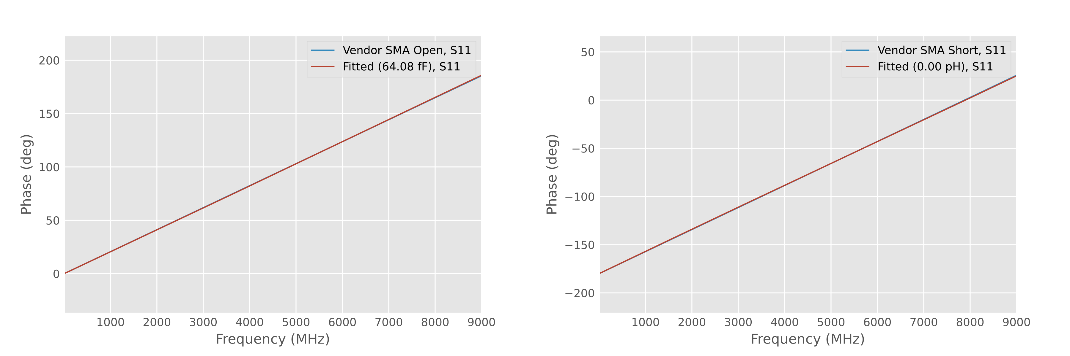 Simulated replication of “zero-parameter
calibration” error results
Simulated replication of “zero-parameter
calibration” error results
Literature shows that the phase shift of a flush coaxial short is less than 1 degree even at 110 GHz (see Appendix 5: Calculation of Short-Circuited Coaxial Line Parasitic Inductance), so L = 0 is of the correct order of magnitude, although the specific value is questionable; the true value might be masked by other experimental errors and not measurable.
As for the capacitance, the conclusion C = 64 fF (20 degrees/9 GHz) is consistent with the conclusion obtained earlier by direct subtraction, as shown below:
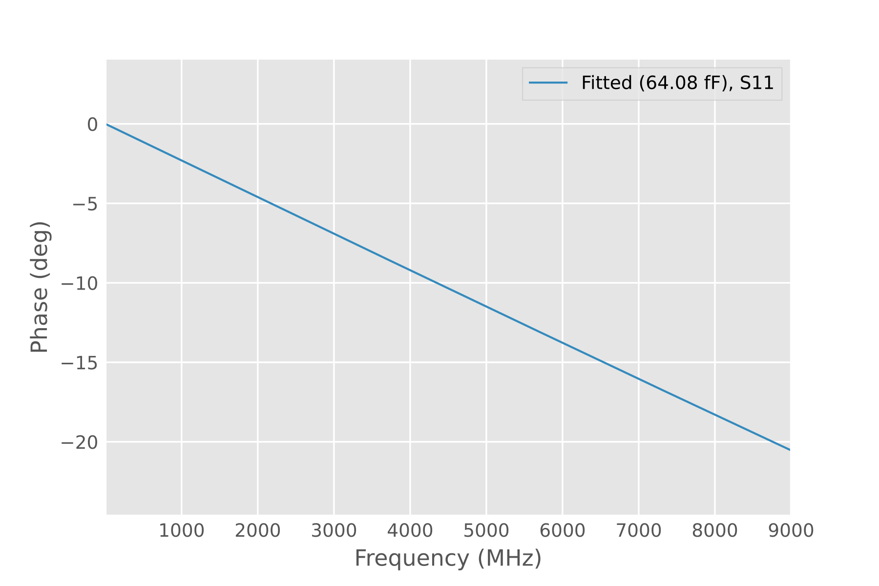 True phase of the open standard inferred
from vendor data
True phase of the open standard inferred
from vendor data
Compared to theoretical and experimental results, this value is still significantly high and its reliability is suspect, but the author cannot further identify the source of error. Due to insufficient information, it cannot be determined that the assumed “mis-calibration” steps described above were exactly the vendor’s operation. Although it is certain that the vendor performed some operation that resulted in a reference plane offset, we cannot know the specific details—for example, the “Port Extension” function can also produce the effect of miscalibration.
Therefore, the specific value of 64 fF inferred from the vendor’s data might also be affected by many factors. The author can only confirm its order of magnitude is correct here, not its precise value.
“Thru” Adapter Effect
As a final hypothesis, the author considered the scenario most favorable to the vendor: perhaps the outrageously large phase shifts of the open and short standards were due to unclear wording, failing to specify the measurement subjects clearly?
We know most connectors have plug and socket variants, and 3.5 mm / SMA are no exception; only a few special connectors (like GR-874 or APC-7) are “genderless.” This means plugs and sockets require separate calibration. In experiments, we almost always need to calibrate coaxial cable plugs, not the sockets on the VNA instrument itself. Due to this dreadful “gender,” a well-equipped lab must bear double the cost, purchasing two sets of calkits for plugs and sockets separately.
 Calibrating SMA ports requires buying two
sets of calkits, money down the drain…
Calibrating SMA ports requires buying two
sets of calkits, money down the drain…
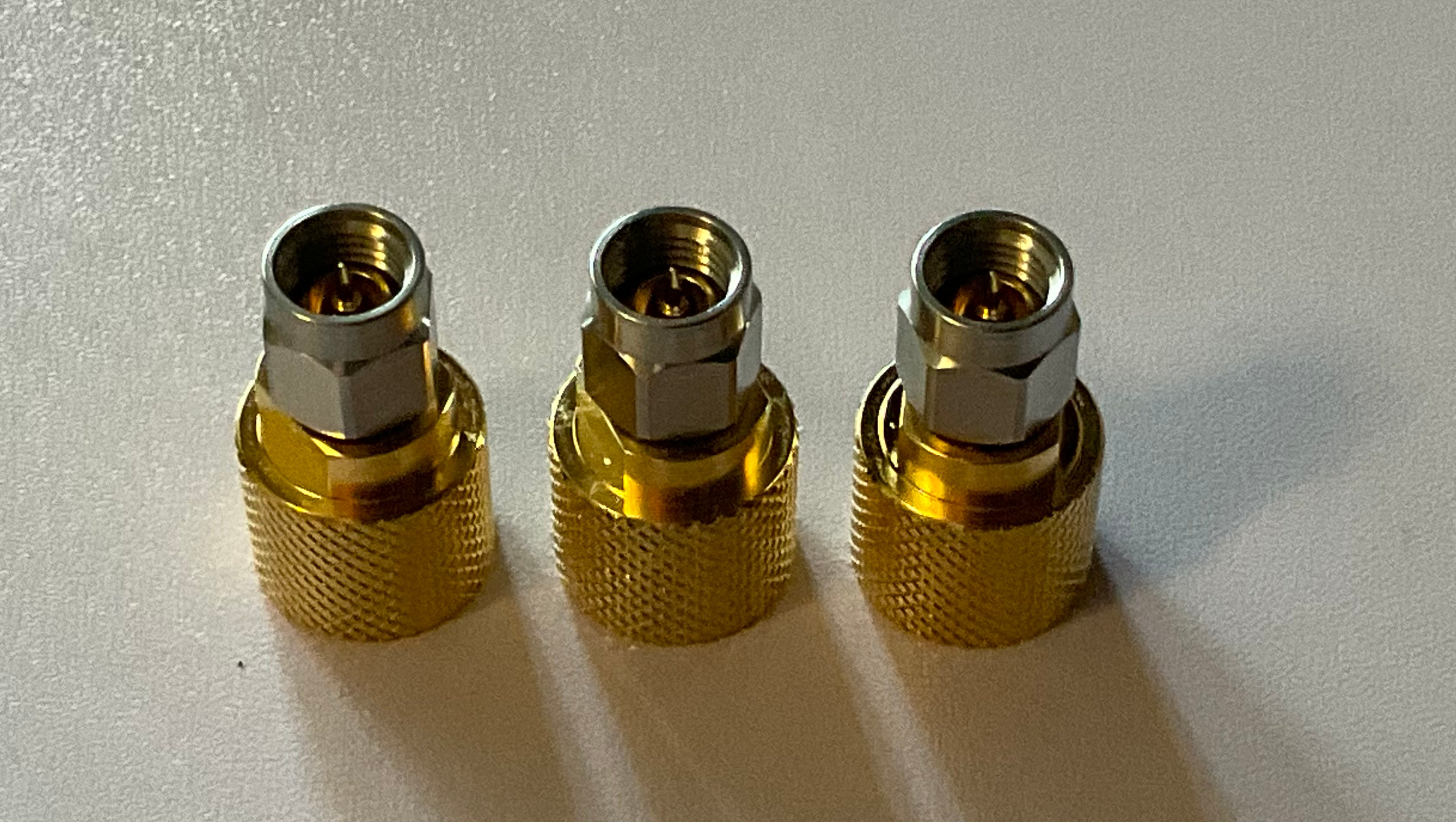
Commonly available generic 3.5 mm / SMA calkits on the market are only available in plug form, not socket form.
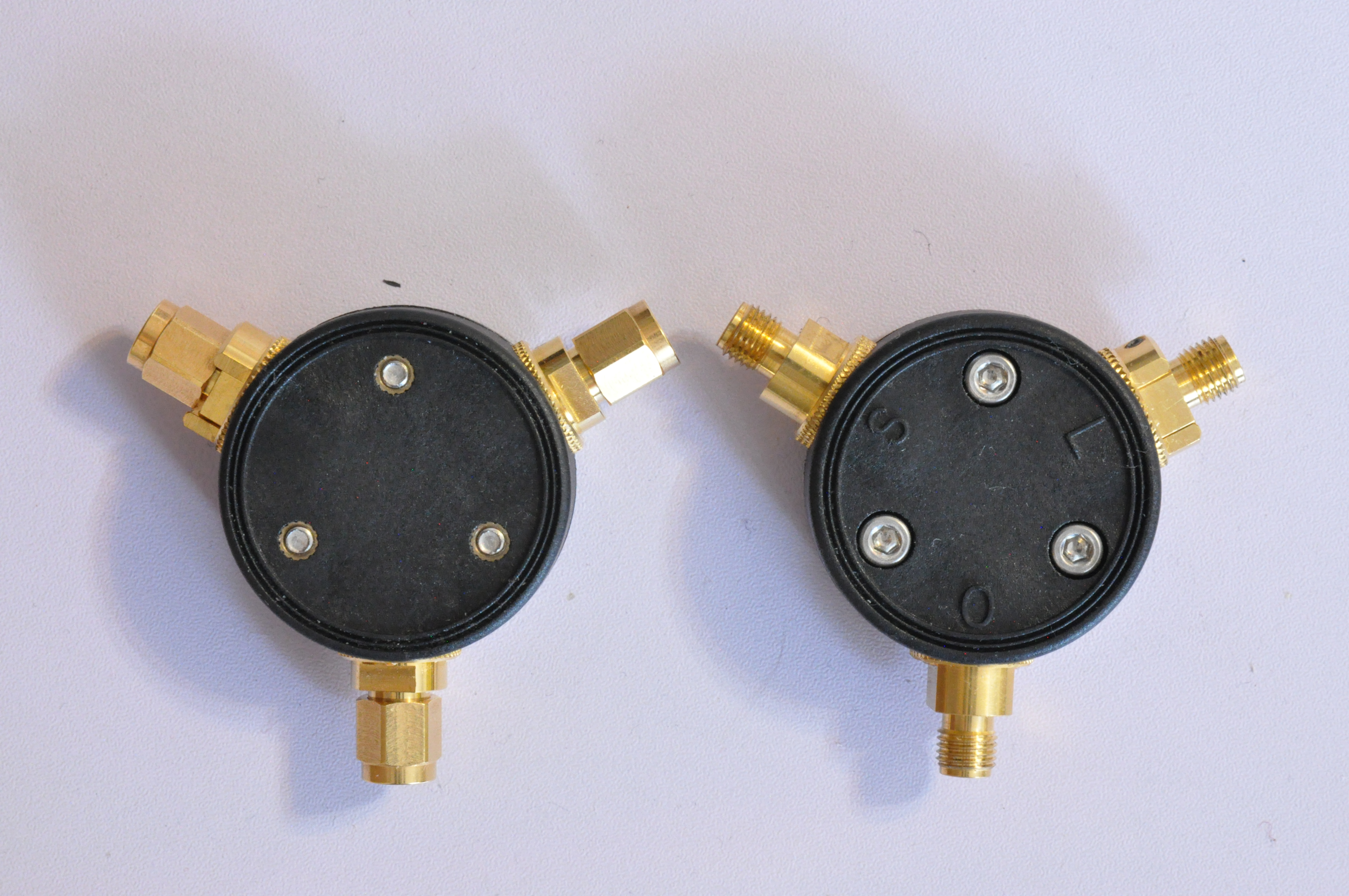
 Generic open, load, short
standards
Generic open, load, short
standards
If we want to connect the generic calkit to a coaxial cable, we must use the Thru adapter included with the generic kit.
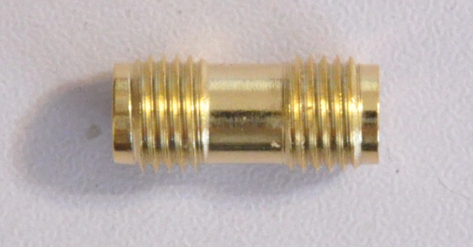 Generic Thru
adapter
Generic Thru
adapter
This introduces a small section of transmission line, which produces a huge phase shift.
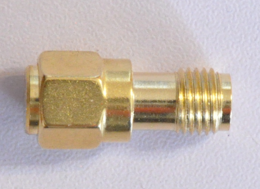 Generic Thru adapter connected
to open standard
Generic Thru adapter connected
to open standard
According to the author’s preliminary test results, the delay of a generic Thru adapter is 47.08 ps, equivalent to a -305 degree phase shift (at 9 GHz). Here, we encounter a completely opposite problem: the vendor’s data shows an error that is instead too small, only 205 degrees, missing by 100 degrees. According to data published by radio amateur Kurt Poulsen (OZ7OU), the shortest generic Thru adapter he has seen has a delay of at least 42.35 ps [23] (phase shift of -274 degrees at 9 GHz).
Therefore, this explanation does not hold, not to mention the completely inexplicable sign error still exists.
We can’t help but feel regret for the vendor: if they had measured the error of the “generic Thru + generic standard” combination, they could have obtained an even more startling calibration error, achieving better marketing effect: up to -305 degrees—such data would have been completely true, reasonable, and fair.
Other Issues
Besides the absurd experimental data, the vendor’s published article contains two other factual errors worth clarifying here.
Misconception About Calibration Results
The vendor believes that after VNA calibration, measuring a set of calkit should yield:
The result for a normal open standard should be a horizontal line at 0 degrees, and for a short standard, a horizontal line at 180 or -180 degrees.
This is incorrect. An ideal open standard’s phase should indeed be a horizontal line at 0 degrees, and a short standard at 180 or -180 degrees. But as we have emphasized at the beginning: perfect open and short standards are unattainable; the phase of real devices must vary with frequency. The purpose of creating a set of calkit is not to create perfect devices “without parasitics” but to create practical devices with stable, known parasitics. Calibration error is not determined by “parasitics” but by the definition data.
The measured phase of normal open and short standards is not always a horizontal line—their phase shift can be arbitrarily large, as long as it matches the theoretical data we have in the definitions. For example, the stock Agilent 85033E open standard must produce a “large phase shift” of 205 degrees at 9 GHz which we know, no more, no less.
 Theoretical data for Agilent 85033E open
standard
Theoretical data for Agilent 85033E open
standard
Only when the calkits lack characterization data, forcing us to assume they are perfect, is the “horizontal line” the desired phase.
Furthermore, the calibration algorithm itself works by forcing the VNA’s readings to match the definitions of the calkit. Therefore, another important conclusion is: if we calibrate the VNA first and then measure this same set of calkit, we will always get perfect theoretical results—here, the calkit is “acting as both player and referee.” Similarly, the measurement result in this case is not a horizontal line but the definition data itself.
Most perplexingly, before publishing this article, the vendor had specifically published an article educating readers [24]:
The open standard you are testing is a capacitor. Since it’s a capacitor, it should lie in the capacitive plane. It obviously won’t be a point, but an arc. Of course, the length of the arc is determined by your frequency range. If the bandwidth is wide, the arc might circle the outer circle several times.
But in the article published two weeks later, the vendor “forgot” this key point from their own article. Did the vendor suddenly lose their memory?
Misconception About Hollow Opens
In another article, The Secret Behind Network Analyzer Calibration Kit Open Standards, the vendor also expressed misconceptions similar to this article’s content, claiming that all hollow open standards are universally untrustworthy [25]:
After introducing the basic parameters of open standards, let’s look at some open standards sold on the market. The figure below shows that some manufacturers provide open standards with no center pin at all, just the housing. How can the capacitance and delay of such open standards be evaluated?
The vendor even once referred to sellers of such open standards as “unscrupulous vendor” in a Taobao product description [26]:
What’s more, many unscrupulous vendor’ open standards are just empty inside. How can parameters be extracted?
Then look at the picture. The photo below shows the HP 11866A APC-7 calkit designed in 1977 [27], [28], whose open standard has no center pin.
![HP 11866A APC-7 calibration kit[28]](https://niconiconi.neocities.org/img/review-of-a-misleading-vendor-article-on-vna-calibration/hp_11866a.jpg) HP 11866A APC-7 calibration kit[28]
HP 11866A APC-7 calibration kit[28]
Similarly, the photo below shows the open standard from the HP 85032B/E calkit, used for calibrating Type-N connectors, which also has no center pin [29], [30]:
![HP 85032B/E Type-N connector open calibration standard[29]](https://niconiconi.neocities.org/img/review-of-a-misleading-vendor-article-on-vna-calibration/hp-85032b-e-open.jpg) HP 85032B/E Type-N connector open
calibration standard[29]
HP 85032B/E Type-N connector open
calibration standard[29]
Is Hewlett-Packard, USA - the predecessor of the company that manufactured the VNA the vendor used for their own experiment—an “unscrupulous vendor”?
The vendor’s unwarranted blanket dismissal of these devices demonstrates that, as a seller of calkits, they are completely unaware of the historical classic “circular waveguide” open standard design. The vendor believes evaluating its capacitance is an impossible task, even questioning readers on how to achieve it, unaware that this was work initially completed during WWII and commercialized by the 1970s.
On one hand, this is understandable: literature indicates that pinless circular waveguide opens were widely used only on APC-7 connectors [31] (most effective, as APC-7 itself is a precision connector), with some application on Type-N connectors as well. Nowadays, they are obsolete technology due to their own limitations. In modern connectors, there indeed exist issues with unstable parasitic parameters, so modern connector open standards are pin-based.
On the other hand, since the vendor’s WeChat slogan is “The core technical team includes PhDs in electromagnetics and microwaves, hoping to provide everyone with the most professional knowledge unavailable elsewhere,” they must enhance their level of knowledge. Before “providing everyone with the most professional knowledge unavailable elsewhere,” they should at least familiarize themselves with the professional knowledge available to everyone in the IEEE database.
An Easter Egg
If we look again at the generic Type-N Open standard the vendor tested and heavily disparaged, we find they look familiar!
Seller’s measured “generic” Type-N open
standard
This is the secret of the generic Type-N calibration standards (first discovered by Kurt Poulsen [OZ7OU]): almost all generic Type-N calibration standards circulating in the Shenzhen market are clone of the HP 85032B/E [23]. The so-called “generic”, “unknown” open standard dusts off a forgotten history: they were actually supported by both electromagnetic theory and practical applications. These clones are still being passed down generation after generation through copying. At the same time, both users and clone manufacturers themselves have long forgotten the original source or its theory of operation.
Ultimately, it became a generic mystery calkit, sold by sellers with no understanding of their electrical characteristics and purchased by buyers with no knowledge of its design. The generic calkit still otherwise works if correctly used, albeit with a poorer tolerance. But almost nobody knows the correct usage today (that is, entering HP 85032B/E’s parameters) because its origin has been forgotten in spite of still being sold everywhere. This is truly terrifying.
This also means that in amateur radio, if we encounter such generic Type-N calibration standards, we can simply input the official definition parameters of the HP85032B/E [22] to achieve a rough calibration with reasonable accuracy.
Conclusion
The vendor correctly demonstrated that if we use “offset” type calkits to calibrate a VNA without entering the definition parameters, the measurement error is obviously huge. On a technical level, the article’s claim is narrowly correct—whether the standards are stock or generic, the use of all-zero parameters will cause the same problem:
The phase deviation of open and short standards from VNA calibration kits without extracted parameters isn’t a simple 5 or 10 degrees. It’s errors of tens, even hundreds of degrees.
However, when presenting the error of generic calkits to readers, the vendor’s method of displaying data was severely misleading. The vendor showcased the error in a specific scenario, leading readers to believe the error is equally large in all scenarios, seriously misleading them. Admittedly, uncharacterized standards must have errors, but this error varies in magnitude depending on the situation.
Ironically, because generic standards are flush standards, they are closer to the ideal assumption than stock “offset” standards. When using the all-zero ideal assumption, their error is actually better than that of stock standards, with the open standard error being only 10-20 degrees (at 9 GHz), not the claimed “tens, even hundreds of degrees.”
Even more ironically: the vendor could have simply tested the generic standards with the “Thru” adapter and reported the results truthfully—their true error would have been even more exaggerated than the vendor’s erroneous data, reaching 300 degrees. Calibrating cable plugs is the most common and important task in RF measurement. The vendor could reasonably claim that generic calkits lead to huge measurement errors in this scenario. Doing so would be objectively true and fair, and subjectively align with the vendor’s commercial interests. Yet, the vendor still chose to publish severely misleading and incorrect test results.
The vendor’s overly absolute and blanket dismissal of hollow open standards in the article also shows unfamiliarity with the history of VNA calibration standards, complete ignorance of “circular waveguide” open standard theory, and lack of awareness of historically classic APC-7 and Type-N open designs. The vendor should enhance their knowledge base.
Furthermore, as this article neared completion, the author rechecked the product description of an inexpensive SMA calkit in the vendor’s Taobao store. There, the vendor backtracked, saying: “If it’s a simple open/short standard with a hollow body, the phase error is almost 10-20 degrees or more” [32], no longer claiming they have errors of “tens, even hundreds of degrees.” This suggests the vendor may have already realized their mistake after the fact, but the original WeChat article was not deleted or corrected.
The author must warm the vendor: if one browses the company’s official website and Taobao product catalog [33], it’s easy to see the products have obviously undergone professional R&D: besides calkits for different connectors, there are also resonator-based permittivity and permeability test systems (the company also claims to have served clients like NVIDIA, BYD, or Tsinghua University). However, the publication of such flawed articles on the company’s WeChat account gives potential customers the impression that the “company managers are ignorant and incompetent,” unnecessarily damaging the product’s reputation.
Finally, the author reminds readers: the basic SOL calibration algorithm of a VNA is by no means a trade secret or magic; its working principles are explained in depth in many manufacturers’ application notes. The algorithm at its core only involves high-school algebra: linear equations with three variables (see Appendix 1: SOL Calibration Algorithm). Open-source software like the scikit-rf library provides complete source code: readers can even write their own scripts to calibrate a VNA without relying on the instrument itself—in fact, this is an excellent way to process experimental data, transparently preserving all raw data. If readers prepare themselves with common measurement knowledge, they won’t be deceived by marketing rhetoric that exploits their ignorance.
As the great physicist Richard Feynman said:
 For a successful technology, reality must
take precedence over public relations, for Nature cannot be
fooled.
For a successful technology, reality must
take precedence over public relations, for Nature cannot be
fooled.
Appendix 0: True Parasitics of Generic Calkits
The previous text has proven the vendor’s data to be completely untrustworthy. So, what is the typical error introduced when using generic calkits?
Preliminary Conclusions
Generic Open, Load, Short
Standards
When using generic calkits to calibrate an SMA socket, the phase error of the generic open standard, compared to an ideal open, is only 5 degrees (at 9 GHz); in the commonly used amateur microwave bands (below 6 GHz), the error is only 3 degrees; and in the amateur VHF/UHF bands, the error is only 0.5 degrees.
 Generic Open Error (SMA Socket
Calibration)
Generic Open Error (SMA Socket
Calibration)
Due to complex technical reasons, the capacitance of the SMA socket might be underestimated, representing merely an “equivalent” capacitance rather than a physical one. Measurements using a 3.5 mm socket yield results closer to the true error. Under these conditions, the measured error remains small: only 10 degrees (at 9 GHz); in the commonly used amateur microwave bands (below 6 GHz), the error is only 6 degrees; and in the amateur VHF/UHF bands, the error is only 1 degree.
 Generic Open Error (3.5 mm Socket
Calibration)
Generic Open Error (3.5 mm Socket
Calibration)
When using a generic Thru adapter to calibrate an SMA plug, the error increases by 50-305 degrees (0-9 GHz) on top of the aforementioned measurement error. Clearly, when calibrating cables, the generic Thru adapter must be compensated for using the correct standard definition.
 Generic Through + Open Error (SMA Plug
Calibration)
Generic Through + Open Error (SMA Plug
Calibration)
As for the generic short standard, for the reasons stated earlier, it is essentially a flush short. Given the author’s current experimental setup (single-port) and instrument limitations, meaningful values cannot be measured and should be approximated as 0. This issue will be further investigated in the future using a better two-port measurement method.
Open Standard Parasitic Capacitance
In a 2014 experiment by radio amateur Kurt Poulsen (OZ7OU) [23], using a VNWA2 analyzer (0-1.3 GHz) [34] and an HP 85033C 3.5 mm calkit [35], the equivalent delay of an unterminated 3.5 mm coaxial socket was measured as 1.32 ps (i.e., 26.40 fF equivalent capacitance). In the author’s own preliminary, unpublished experiments in 2025, using a VNA6000 analyzer (0-6 GHz) and an HP 85033E 3.5 mm calkit, various 3.5 mm coaxial sockets were measured under different conditions. The equivalent capacitance of the “generic” short open (most common) was found to be between 24.60-31.53 fF; the “generic” long open between 23.10-29.76 fF; and the unterminated socket between 22.40-29.20 fF.
The author’s preliminary test results are shown in the table below. The adapter models used were [36], [37], [38], [39].
| 3.5 mm | HP 85052-60003 | Unterminated | 26.40 fF | D (Low) | OZ7OU |
| 3.5 mm | Keysight 5061-5311 | Short Open | 24.60 fF | C (Medium) | Author |
| 3.5 mm | Keysight 5061-5311 | Long Open | 23.10 fF | C (Medium) | Author |
| 3.5 mm | Keysight 5061-5311 | Unterminated | 22.40 fF | D (Low) | Author |
| 3.5 mm | WITC 1011-01-SA2 | Short Open | 31.53 fF | C (Medium) | Author |
| 3.5 mm | WITC 1011-01-SA2 | Long Open | 29.76 fF | C (Medium) | Author |
| 3.5 mm | WITC 1011-01-SA2 | Unterminated | 29.20 fF | D (Low) | Author |
| SMA | EastSheep SMA-JKG | Short Open | 13.67 fF | D (Low) | Author |
| SMA | EastSheep SMA-JKG | Long Open | 10.55 fF | D (Low) | Author |
| SMA | EastSheep SMA-JKG | Unterminated | 9.57 fF | F (Worst) | Author |
| 2.92 mm | WITC 4021-01-SA1 | Short Open | 11.03 fF | D (Low) | Author |
| 2.92 mm | WITC 4021-01-SA1 | Long Open | 10.57 fF | D (Low) | Author |
| 2.92 mm | WITC 4021-01-SA1 | Unterminated | 10.46 fF | F (Worst) | Author |
According to academic literature, the open-end capacitance of an ideal 3.5 mm air coaxial line should be approximately 30-40 fF; however, the experimental data is significantly lower, with a maximum deviation of -20 fF from the ideal value.
The author believes that measuring the open-end capacitance of coaxial connectors is affected by various factors. The 22.40-31.53 fF measured here may merely represent the “equivalent” open-end capacitance of the connector when the port is unterminated after an SOL calibration, rather than the true physical open-end capacitance. The electrical parameters of a coaxial connector in the “unconnected” and “connected” states may not be consistent: after calibration using calkits, we establish the error of the connector in the “connected” state because the connector actually makes mechanical contact with the calkit (or future DUT), and their connector designs are similar; however, we cannot extrapolate the same error term to the connector in the “unconnected” state. Therefore, using the “equivalent” open-end capacitance of the unconnected port to calibrate the instrument can be accurate for future measurements in the “connected” state, but the capacitance value itself in the “unconnected” state may not be accurate.
The situation for SMA and 2.92 mm sockets is more complex. Based on the author’s own experiments, their equivalent capacitance is around 10 fF, showing significant deviation from theoretical values. These experiments indicate that the parasitics of a coaxial open are not stable, depending not only on themselves but also on the mating connector, making their parasitic effects complex. This is likely the reason hollow open standards are no longer used for SMA/3.5 mm standards. As for the measured 10 fF data, it may not be the true value but rather a result of additional parasitic effects caused by using a 3.5 mm calkit to calibrate SMA and 2.92 mm ports, leading to over-compensation during calibration and deviation in the open capacitance result. For a detailed discussion of this issue, see Appendix 4: Calculation of Open-Ended Coaxial Line Fringe Capacitance.
Based on the above assessment, the author considers the physical meaning of all 3.5 mm data to be “C (Medium)”, and all 2.92 mm/SMA data to be “D (Poor)”. Additionally, unterminated opens are susceptible to influence from surrounding objects, downgrading their physical meaning by one level to “D (Low)” and “F (Worst)” respectively.
“Thru” Adapter Delay
Commonly available generic 3.5 mm / SMA calkits on the market are only available in plug form, not socket form. However, the vast majority of experiments are not conducted directly on the VNA ports but through test cables. If we want to connect generic calkits to a coaxial cable, we must use the Thru adapter included with the generic kit. This introduces a small section of transmission line, which produces a significant phase shift. The Thru adapter delay must be compensated for to obtain correct results. Otherwise, it will cause an error of 300 degrees.
Generic Thru
Adapter
According to data published by radio amateur Kurt Poulsen (OZ7OU) in 2014, a common inexpensive generic Thru adapter has a delay of approximately 42.35 ps [40]. Based on the author’s limited testing, its delay is 47.08 ps.
Recommended Values
Based on the above test results, the author recommends the following parameters for generic calkits. Due to current experimental limitations, the very low loss of the calkits cannot be measured (on the order of 0.01 dB), so all loss-related values should be set to 0. Similarly, due to large phase measurement errors, stable polynomial interpolation cannot be achieved, and only the simplest linear fitting is possible; therefore, C₁, C₂, C₃ should all be set to 0. Finally, the inductor parameters L₀, L₁, L₂, L₃ should also be set to zero.
| 3.5 mm Socket | No | Short Open | 0 ps | 28.065 fF |
| 3.5 mm Socket | No | Long Open | 0 ps | 26.430 fF |
| SMA Socket | No | Short Open | 0 ps | 13.670 fF |
| SMA Socket | No | Long Open | 0 ps | 10.550 fF |
| SMA Plug | Yes | Short Open | 47.08 ps | 13.670 fF |
| SMA Plug | Yes | Long Open | 47.08 ps | 10.550 fF |
All the above results are preliminary. They are published only to provide the amateur radio community with approximate values as soon as possible, offering better test data than the ideal assumption. These data have not yet undergone rigorous verification and possess the various defects mentioned above. For example, the quality of the SMA data here is significantly inferior in comparison to 3.5 mm connectors. The author plans to conduct more experiments with different methods (such as the more accurate parallel resonance method), and with an increased sample size.
Warning
Readers must also be warned that commonly available generic calkits on the market actually violate the SMA connector design specification.
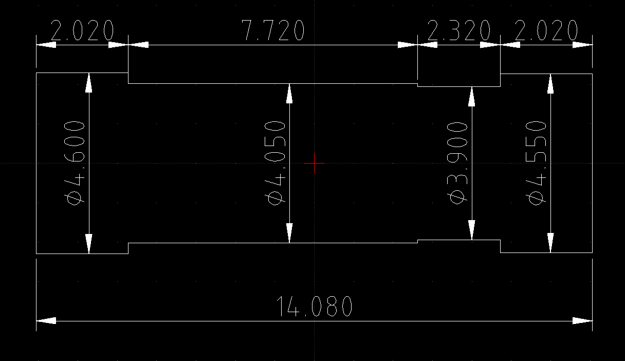
It has been fully confirmed that one end of the generic Thru adapter violates industrial standards: one end has an inner diameter of 4.600 mm, while the other end is only 4.550 mm, violating the requirements in IEC 61169-15 [17]. This might be an intentional design to prevent simultaneous rotation of both sides, by increasing friction on one end. This design makes the Thru adapter prone to seizing, easily damaging cables or VNA ports.
 Measurement data of the generic
Thru adapter
Measurement data of the generic
Thru adapter
Furthermore, the generic short standard is suspected of having an overlong center pin, pending further confirmation.
If other readers wish to test generic calkits to reproduce this experiment, be sure to prepare dedicated sacrificial cables and sacrificial adapters to avoid damaging expensive cables or instrument ports. It is worth noting that these problems are not unique to generic calkits but are common issues with inexpensive commercial-grade SMA connectors; caution is needed when using any commercial-grade SMA device. When using expensive instruments or accessories, all connectors must be checked with an “SMA interface gauge”. See the author’s other article for details: SMA Connector Pin & Dielectric Tolerances.
For radio amateurs with the means, it is strongly recommended to discontinue using the generic Thru adapter and instead purchase a separate high-quality Thru adapter with a flange. This type of Thru adapter has a longer delay than the generic one, and direct replacement would increase the error. However, one can first use the data above with the generic Thru adapter to temporarily calibrate the VNA. Based on this, measure the phase at the highest measurement frequency for both the “Generic Thru + Open” and the “Flanged Thru + Open” combinations, calculate the phase difference between them Δϕ=ϕnew−ϕold, and then calculate Δt using the formula below to calibrate the new delay data.
Δt=Δϕ−720∘f
Appendix 1: SOL Calibration Algorithm
The measurement data from a VNA can be viewed as a cascade of a forcibly imposed “error circuit” and the Device Under Test (DUT). Any true reflection coefficient Γ is modified by a hypothetical Error Box, resulting in a distorted Γ′ [41], [42].
 Error model for single-port VNA
measurement
Error model for single-port VNA
measurement
Like any two-port network, the Error Box consists of S-parameters (e.g., S11, S22, S12, S21), but these are hidden from the operator. It contains errors introduced by the signal path (e.g., reflections, phase shifts) and also linear errors from the VNA’s own receivers. If the complete S-matrix of the error box can be deduced, the measurement errors can be eliminated.
According to the cascade formula for S-parameters (Textbook Chapter 4.5 [43]), the relationship between the measured result and the ideal result is:
Γ′=S11−(S11S22−S21S12)Γ1−S22Γ
The four S-parameters of the error box are mixed with the DUT’s reflection coefficient, with cross-multiplication terms in particular, making direct solution seem difficult. However, we do not need to determine each S-parameter individually but can describe the overall effect of the error box on the measurement result.
By introducing the following coefficients and variables, the measurement equation can be linearized:
m1=1x1=S11m2=ΓΓ′x2=S22m3=−Γx3=S11S22−S21S12
The coefficients on the left are calculated from the calkit’s definitions and the measurement results, both are completely known; the variables on the right are combinations of the unknown error box’s S-parameters, describing the overall error.
Substituting the new variables, the original equation can be rewritten as:
Γ′=x1−x3Γ1−x2ΓΓ′−ΓΓ′x2=x1−Γx3Γ′−m2x2=m1x1+m3x3Γ′=m1x1+m2x2+m3x3
Note that the number of variables is reduced from 4 to 3 after simplification. The intuitive explanation is: the attenuation of the reflected signal could be due to attenuation on the forward or on the reverse path; the contributions of the error box’s transmission coefficient from port 1 to port 2, S12, and from port 2 to port 1, S21, cannot be distinguished solely by single-port measurements. Therefore, effectively only three error terms exist. Some literature applies normalization (set S21=1 [42]) or assumes S21=S12 (reciprocal network assumption, e.g., textbook [41] p. 30).
If we measure three calibration standards with arbitrary known reflection coefficients Γ1, Γ2, Γ3, we obtain three measurement results Γ1′, Γ2′, Γ3′. A system of equations can be established at each measurement frequency point f:
m11x1+m12x2+m13x3=Γ1′m21x1+m22x2+m23x3=Γ2′m31x1+m32x2+m33x3=Γ3′
After solving for x1, x2, x3, substitute them into the original equation to calculate the error-free ideal Γ. Solving this system of three linear equations requires only high-school algebra.
Note that in principle, we can use any calibration standards with known characteristics, but their positions on the complex plane should not be too close. Otherwise, an ill-conditioned situation arises where two measurement results are very similar, causing the algorithm to lose numerical stability (the system’s condition number becomes large). This is also why open and short standards are commonly used—regardless of frequency, their arguments always differ by 180 degrees.
Appendix 2: Reverse Engineering Vendor Data
To analyze the measurement data provided by the vendor, the raw data needs to be reverse-engineered from the screenshots. Credit is due to the vendor for thoughtfully providing three markers, with phase values at three frequency points accurate to three decimal places, which greatly aided our extraction work.
Manually Writing Touchstone Files
In the field of RF measurement, the industry standard for S-parameters is the Touchstone format. We first recover the marker values into machine-readable data by manually writing .s1p files.
The manually written file is as follows. Note that the first line starting with # in a Touchstone file is metadata, not a comment, and cannot be omitted. Real comments start with !.
sma_open.s1p:
# GHz S MA R 50 !freq magS11 angS11 0.000 1.000 0.000 3.000 1.000 61.881 6.000 1.000 123.88 9.000 1.000 185.39The Touchstone file itself supports many data formats; the most commonly used is usually the RI (Real Imaginary) format, which is most convenient for complex number programming. However, since the vendor’s original data is given in angles, we can use the MA (Magnitude Angle) format.
The original image only includes exact values for three data points (3 GHz, 6 GHz, 9 GHz). Considering that interpolation is often automatic in many RF simulation software, but extrapolation is rarely used, we manually add an ideal value at 0 GHz here to facilitate subsequent interpolation work. Additionally, the published screenshots contain no magnitude information. Since we know the typical loss of coaxial open and short standards is very small, on the order of 0.001 dB, we approximate them as ideal and lossless here.
sma_open.s1p can be opened and analyzed directly by any circuit simulation tool.
scikit-rf Interpolation
Here, we use the powerful Python RF library scikit-rf to perform linear interpolation on the data, thus recovering the original data.
interp.py:
import sys import pathlib import skrf from matplotlib import pyplot as plt skrf.stylely() # apply skrf's built-in matplotlib style plt.figure(figsize=(6.40, 4.80)) # 4:3 image # open Touchstone file path = pathlib.Path(sys.argv[1]) network = skrf.Network(path) # linear interpolation from 1-9000 MHz, 1001 points, polar mode new_freq = skrf.Frequency(1, 9000, 1001, unit='MHz') new_network = network.interpolate(new_freq, coords="polar") # Use the original filename (without extension) plus "_interp" suffix # as the new filename, scikit-rf automatically adds the s1p extension. new_network.write_touchstone(path.stem + "_interp") # Display phase plot (unwrapped phase) new_network.plot_s_deg_unwrap() plt.show()Next, just enter python3 interp.py sma_open.s1p, and the program will automatically output sma_open_interp.s1p in the same path. A standard complex format file is generated:
! Created with skrf (http://scikit-rf.org). # MHz S RI R 50.0 !freq ReS11 ImS11 1.0 0.9999999351967374 0.000360009057032283 9.999 0.9999935209766595 0.00359972286477426 18.998 0.9999766110378859 0.0068393988905928755 27.997 0.9999492055578996 0.01007900313153959 ... 8991.001 -0.9958757089624796 -0.09072801275503896 9000.0 -0.9955783744389298 -0.09393455354414477Finally, let’s see how the interpolation effect is? Perfect!
Some might say: Couldn’t we use Euler’s formula to construct complex data points directly with scikit-rf, avoiding the unnecessary step of manually writing Touchstone files? Indeed. But I want to show everyone that Touchstone files are not mysterious and can be written entirely by hand—the more technical knowledge one has, the less likely one is to be deceived.
Other Data
Following the same method, the information from all four screenshots was manually entered in the same way:
sma_short.s1p
# GHz S MA R 50 !freq magS11 angS11 0.000 1.000 -180.00 3.000 1.000 -111.51 6.000 1.000 -43.160 9.000 1.000 25.751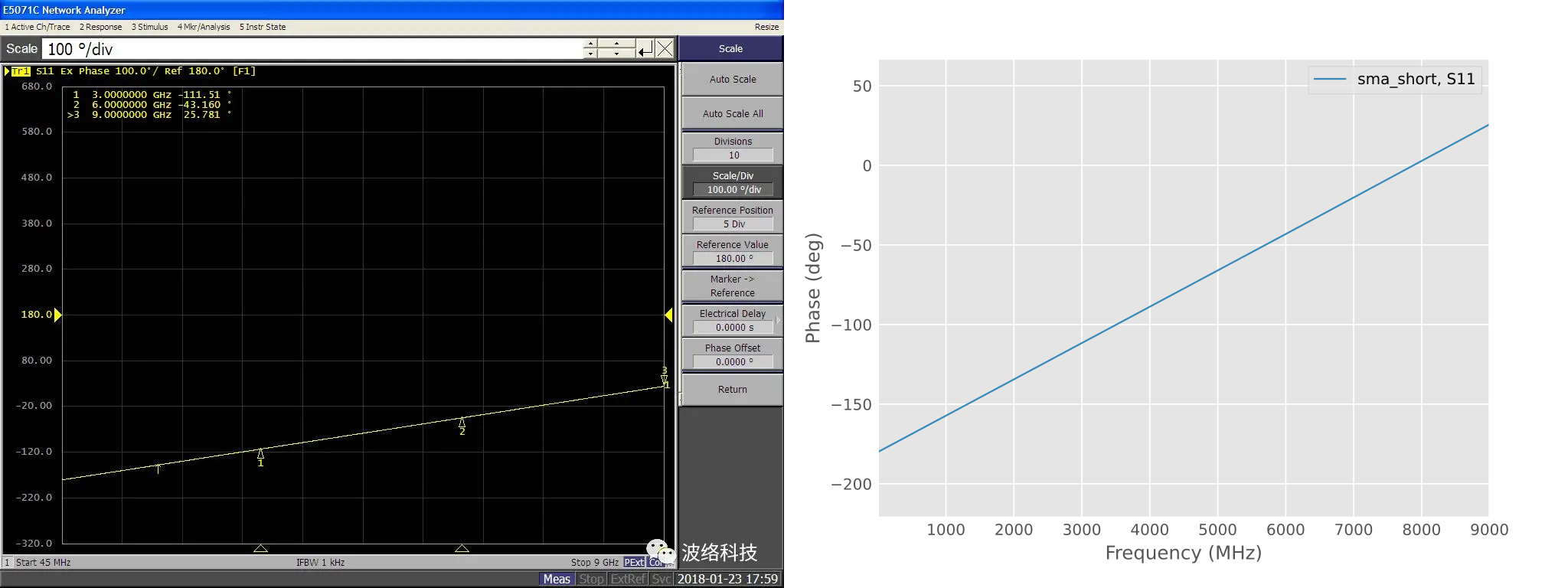
n_open.s1p
# GHz S MA R 50 !freq magS11 angS11 0.000 1.000 0.000 3.000 1.000 83.933 6.000 1.000 166.21 9.000 1.000 250.31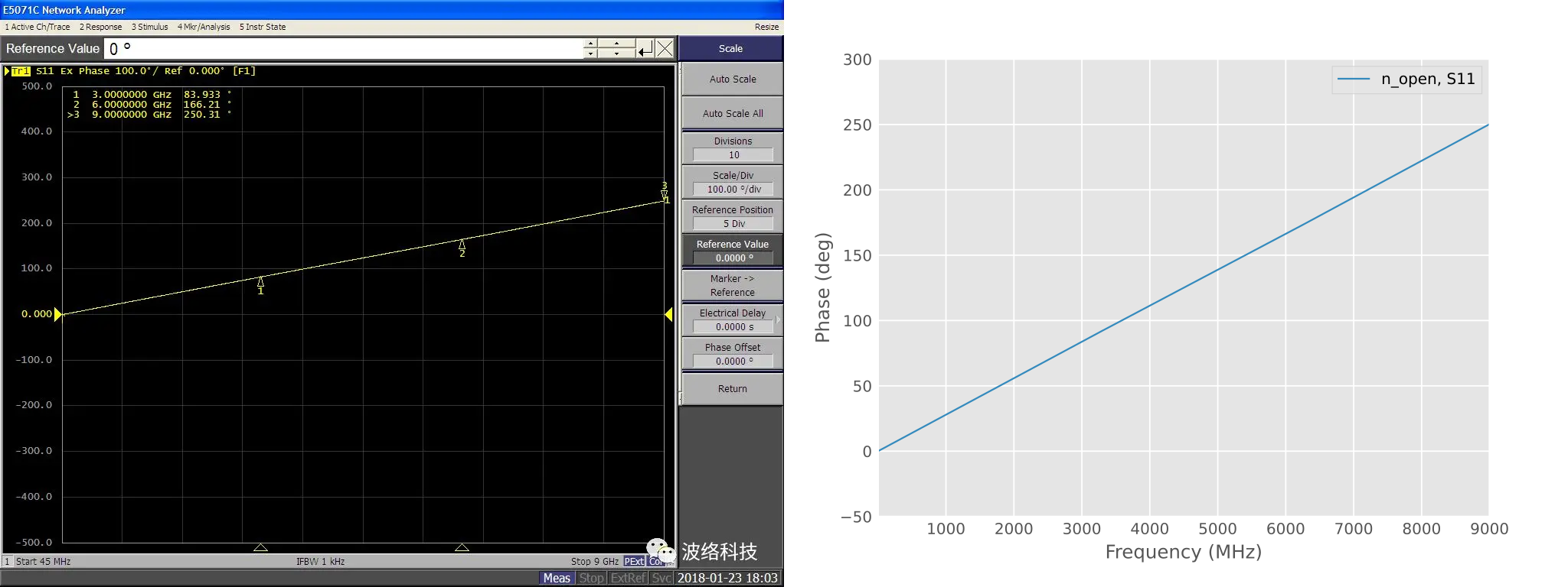
n_short.s1p
# GHz S MA R 50 !freq magS11 angS11 0.000 1.000 180.00 3.000 1.000 149.97 6.000 1.000 123.19 9.000 1.000 97.211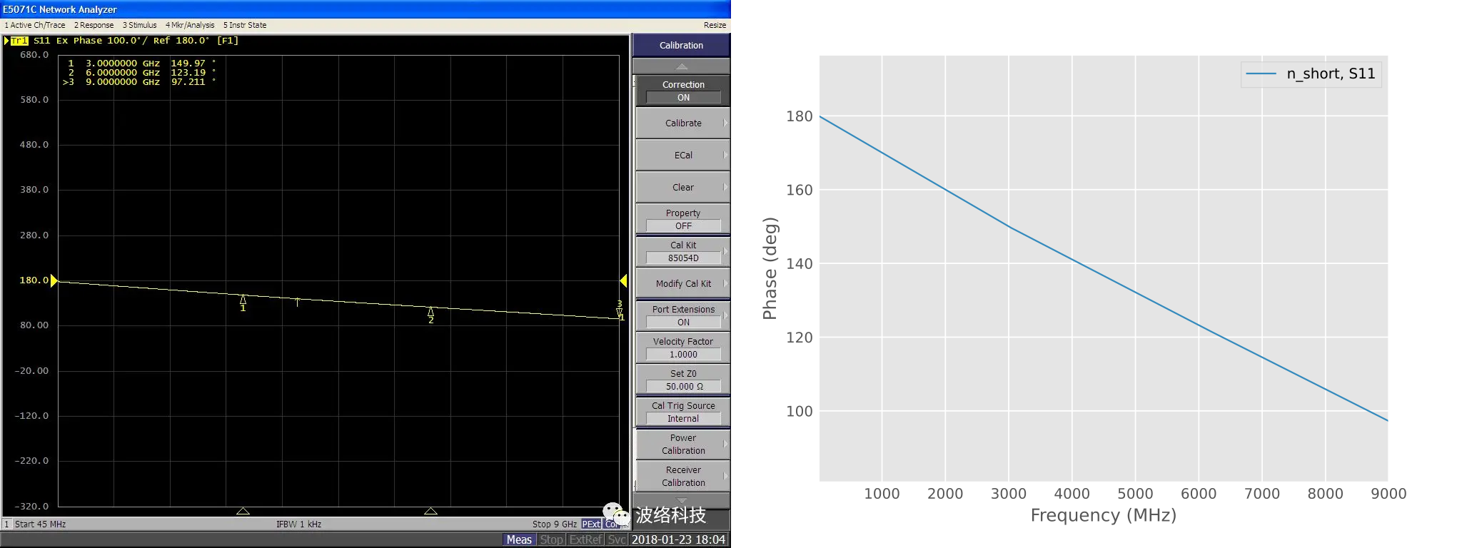
Appendix 3: Equivalent Circuits of Calibration Standards
Content in this section was previously published by the author in the scikit-rf official documentation and has been abridged here. For questions, please refer to the full documentation [44]. Readers may also consult more authoritative original references [45], [46], [47].
Model
The calibration data for standards can be provided directly as raw data (measured S-parameter files) or via equivalent circuits. The equivalent circuit for a calibration standard consists of a transmission line segment in series with a capacitor or inductor, as shown below:
Equivalent circuit model of calibration
standards
These parameters include (some can be omitted if requirements are not stringent):
- Offset delay: The electrical delay of the transmission line, in picoseconds (ps).
- Offset loss: The loss of the transmission line at 1 GHz, in Gigaohms per second (GΩ/s). This unit may seem strange but is quite clever. In microwave measurement, a transmission line is a delay line; length and time are interchangeable. The electrical length of a transmission line segment can be expressed in length units (meters) or time units (seconds), which are equivalent. However, the speed of light differs in various media. If physical length is used, the model requires relative permittivity as an additional parameter, meanwhile delay is always unambiguous in signal measurement (when dispersion can be neglected).
- Offset Z₀: The characteristic impedance neglecting transmission line loss, a real number.
- Parasitic capacitance/inductance (C/L): Varies with frequency, given by a cubic polynomial: y(f)=a0+a1f+a2f2+a3f3.
The standard propagation constant γl and complex characteristic impedance Zc of the transmission line can be obtained from the following formulas:
αl=offset loss⋅offset delay2⋅ offset Z0f109βl=2πf⋅offset delay+αlγl=αl+jβlZc=offset Z0+(1−j)offset loss2⋅2πff109
Note: The length l in γl is normalized, set l=1.
For calculation, first convert the standard parameters to the transmission line’s propagation constant and characteristic impedance, then calculate the two-port S-matrix of the transmission line. Finally, substitute the capacitance/inductance parameters into the polynomial to obtain the one-port S-parameters for the capacitor/inductor at each frequency. The complete S-parameters of the standard are obtained by cascading the transmission line with the one-port S-parameter.
In standard SOL calibration, usually only the open and short are modeled. The standard load is assumed ideal (Γ=0, angle meaningless) and is not modeled further.
Case Studies
The vendor claimed to have compared generic calkits with two sets of Keysight OEM calkits. For further analysis in this article, it is necessary to use the method above to reconstruct the original parameters of these calkits.
Keysight 85033E Plug
This is a 3.5 mm, 50 Ω port calkit, frequency range 0 - 9 GHz. Its pin (plug) type standard definitions are:
| C₀ | 10⁻¹⁵ F | 49.433 | |
| C₁ | 10⁻²⁷ F/Hz | -310.13 | |
| C₂ | 10⁻³⁶ F/Hz² | 23.168 | |
| C₃ | 10⁻⁴⁵ F/Hz³ | -0.15966 | |
| L₀ | 10⁻¹² H | 2.0765 | |
| L₁ | 10⁻²⁴ H/Hz | -108.54 | |
| L₂ | 10⁻³³ H/Hz² | 2.1705 | |
| L₃ | 10⁻⁴² H/Hz³ | -0.01 | |
| Offset Z₀ | Ω | 50 | 50 |
| Offset Delay | ps | 29.2 | 31.8 |
| Offset Loss | GΩ / s | 2.2 | 2.36 |
Open standard frequency response:
Short standard frequency response:
Keysight 85032F Plug
This is an Type-N, 50 Ω port calkit, frequency range 0 - 9 GHz. Its pin (plug) type standard definitions are:
| C₀ | 10⁻¹⁵ F | 89.939 | |
| C₁ | 10⁻²⁷ F/Hz | 2536.80 | |
| C₂ | 10⁻³⁶ F/Hz² | -264.99 | |
| C₃ | 10⁻⁴⁵ F/Hz³ | 13.40 | |
| L₀ | 10⁻¹² H | 3.3998 | |
| L₁ | 10⁻²⁴ H/Hz | -496.4808 | |
| L₂ | 10⁻³³ H/Hz² | 34.8314 | |
| L₃ | 10⁻⁴² H/Hz³ | -0.7847 | |
| Offset Z₀ | Ω | 50 | 49.992 |
| Offset Delay | ps | 40.856 | 45.955 |
| Offset Loss | GΩ / s | 0.93 | 1.087 |
Open standard frequency response:

Short standard frequency response:
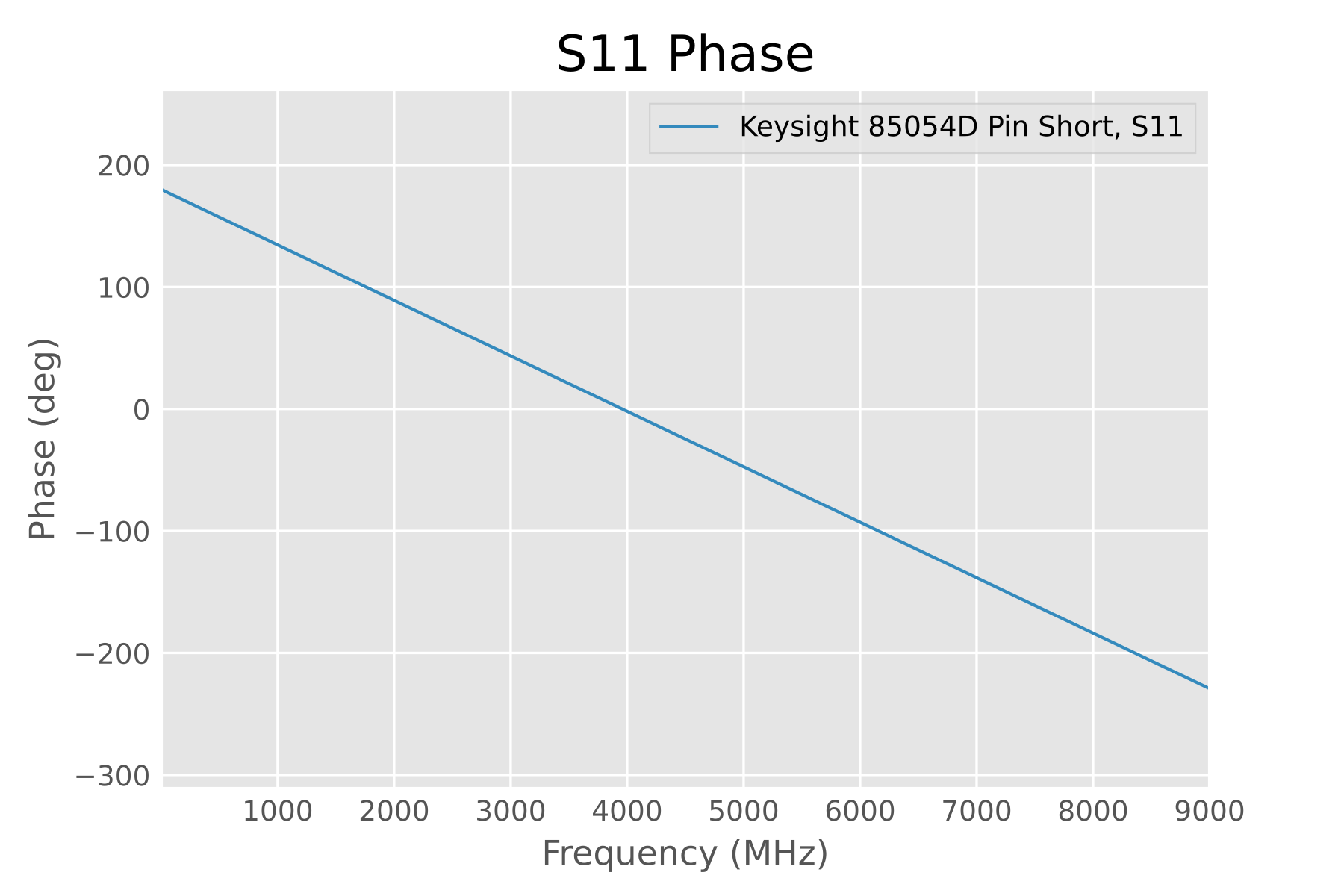
Keysight 85054D Plug
This is an Type-N, 50 Ω port calkit, frequency range 0 - 18 GHz. Its pin (plug) type standard definitions are:
| C₀ | 10⁻¹⁵ F | 89.939 | |
| C₁ | 10⁻²⁷ F/Hz | 2536.80 | |
| C₂ | 10⁻³⁶ F/Hz² | -264.9901 | |
| C₃ | 10⁻⁴⁵ F/Hz³ | 13.40 | |
| L₀ | 10⁻¹² H | 0.7563 | |
| L₁ | 10⁻²⁴ H/Hz | 459.8799 | |
| L₂ | 10⁻³³ H/Hz² | -52.429 | |
| L₃ | 10⁻⁴² H/Hz³ | 1.5846 | |
| Offset Z₀ | Ω | 50 | 50 |
| Offset Delay | ps | 57.993 | 17.817 |
| Offset Loss | GΩ / s | 0.93 | 1.1273 |
Open standard frequency response:
Short standard frequency response:
Code
See Code 0: Calkit Parameter Generation.
Appendix 4: Calculation of Open-Ended Coaxial Line Fringe Capacitance
If a coaxial transmission line is simply truncated, its parasitic capacitance is influenced by the outer conductor thickness, cable radiation, and surrounding objects, making it poorly defined. This structure is typically not used for calculation.
The commonly calculated structures for open-ended coaxial lines are the following cases.
First, the “infinite flange” case, where the outer conductor extends perpendicular to the cable direction, often used for coaxial dielectric probes.
![Infinite Flange[48]](https://niconiconi.neocities.org/img/review-of-a-misleading-vendor-article-on-vna-calibration/grant-probe-geometry.png) Infinite Flange[48]
Infinite Flange[48]
Second, the “coaxial transition to circular waveguide below cutoff” case, where the “outer conductor extends parallel to the cable direction,” often used in metrology standards. The assumptions differ, and the calculation results vary slightly.
Coaxial transition to circular waveguide
below cutoff[5]
For an ideal 3.5 mm coaxial transmission line, the theoretical value of the fringe capacitance is 30-40 fF, although experimental values show significant deviation, discussed in the next section.
Applicability to Coaxial Connectors
Historically, pinless circular waveguide opens were widely used on APC-7 connectors. The HP 11866A designed in 1977 used a pinless circular waveguide [27], [28]. Academic literature also shows high agreement between its theoretical calculations and experimental capacitance values [31]. According to product manuals, the calibrated capacitance of open standards for several historical HP instruments also highly agreed with theoretical values. For example, the open standard capacitance for the HP 4191A RF impedance analyzer was was 82 fF, while the theoretical calculation value was 79.70 fF (see instrument specification on page 32 of Hewlett-Packard Journal [49]).
For Type-N connectors, calibration is more complex due to the misaligned reference planes of the inner and outer conductors [16]. However, HP did indeed release the 85032B/E calkit [30] based on the same principle, also using a circular waveguide open. Notably, Kurt Poulsen (OZ7OU) discovered that most generic Type-N calibration standards circulating on the market are clones of the HP 85032B/E [23]. Without definition parameters, one can borrow the HP 85032B/E parameters—this shows the historical widespread use and significant influence of the latter calkit.
However, circular waveguide open standards have almost never been used on 3.5 mm/SMA connectors. In [50], the author mentions that inserting the center pin itself alters the port’s electrical characteristics. To solve this problem, the center conductor should be filled with dielectric, or a short transmission line segment should be connected in front of the open standard. The author speculates that precisely because the reference planes for the pinned and pinless states are not interchangeable, cavity opens based on the circular waveguide principle fell out of use. For example, the HP 85033C open standard [35] was a product of the transition from circular waveguide opens to pinned opens—it still contained a hollow coaxial connector but had to be used with a “center conductor extender,” which had to be manually inserted. This was meant to mimic the effect of the inserted center pin, making the port’s operating state during calibration consistent with that during actual measurement.
![HP 85033C open standard[35], hollow open must be used with center conductor extender](https://niconiconi.neocities.org/img/review-of-a-misleading-vendor-article-on-vna-calibration/85033c-open.png) HP 85033C open standard[35], hollow open must be
used with center conductor extender
HP 85033C open standard[35], hollow open must be
used with center conductor extender
Through experimentation, the author found significant deviations between the experimental values of circular waveguide open capacitance for both 3.5 mm and SMA connectors and the theoretical values below. Literature indicates that parasitic effects between coaxial connectors are exceptionally complex.
Take step capacitance [51], [52], [53] as an example: when two transmission lines of different physical sizes are connected in series, signal reflection occurs at the discontinuity. However, this reflection cannot be fully explained by characteristic impedance Za≠Zb—in fact, even if the Z0 at both ends is the same, the electromagnetic field remains discontinuous here, causing signal reflection. In circuit terms, this effect is equivalent to a small parasitic capacitance. This was studied by Whinnery in 1944 [7] and calculated by Somlo to five significant figures in 1967 [9].
![Parasitic capacitance between two transmission lines[7]](https://niconiconi.neocities.org/img/review-of-a-misleading-vendor-article-on-vna-calibration/step-capacitance.png) Parasitic capacitance between two
transmission lines[7]
Parasitic capacitance between two
transmission lines[7]
In 1994, HP engineer Pollard used simulation to confirm that this phenomenon also occurs when connecting 3.5 mm, SMA, and 2.92 mm connectors to each other and provided typical values [52].
![Step capacitance for 3.5 mm to 2.92 mm connector[52]](https://niconiconi.neocities.org/img/review-of-a-misleading-vendor-article-on-vna-calibration/2.92-3.5-step.png) Step capacitance for 3.5 mm to 2.92 mm
connector[52]
Step capacitance for 3.5 mm to 2.92 mm
connector[52]
There is reason to suspect the author’s experiment was affected by this effect: when using a 3.5 mm calkit to calibrate an SMA port, this additional step capacitance must cause the parasitic capacitance to be overestimated. When we remove the calkit and try to measure the parasitic capacitance of the empty SMA port, this overcompensation causes the experimental value to be low. However, the magnitude is still insufficient to fully explain the experimental phenomenon: besides step capacitance, effects like center pin depth tolerance [55] also exist. This issue requires further study.
Based on the above experimental facts, when applying theoretical open-end capacitance results to SMA/3.5 mm coaxial connectors, these methods should be considered estimates, not precise values.
Gajda-Stuchly Model
For the “infinite flange” case, Gajda and Stuchly performed calculations in 1983 using the Finite Element Method (FEM) and the Method of Moments (MoM) [13].
For Z0=50Ω coaxial lines in vacuum and PTFE, with the end in vacuum, the low-frequency fringe capacitances are respectively:
Cvac,vacϵ0(b−a)∈[4.076,4.311] F/mCPTFE,vacϵ0(b−a)∈[2.38,2.48] F/m
- ϵ0 is the permittivity of vacuum.
- (b−a) is the difference between outer and inner conductor radii, in meters (m).
- Relative permittivity of PTFE ϵr,line=2.05
- Lower and upper bounds are MoM and FEM calculation results, respectively.
Applicability: This low-frequency result is valid only for Z0=50Ω, when the outer conductor is widened to satisfy the “infinite flange” condition, and the cable end is in vacuum. For other Z0 values and media, recalculate using lookup tables.
Example: For an ideal vacuum line (3.5 mm/1.52 mm), capacitance is between 35.73 fF and 37.79 fF; for an ideal PTFE coaxial line (4.13/1.25 mm), capacitance is between 30.35 fF and 31.62 fF.
Somlo Model
For the “circular waveguide below cutoff” case, P. I. Somlo provides the most authoritative data.
In 1967, P. I. Somlo used the mode-matching method and a CDC 3600 mainframe computer to calculate the parasitic parameters of coaxial cable geometric discontinuities to five significant figures, far exceeding experimental accuracy and almost closing the issue. It remains the standard reference data today. General calculations and data were published in [9], with the open-end equivalent capacitance problem specifically addressed in [10].
![Data from Somlo’s paper[10]](https://niconiconi.neocities.org/img/review-of-a-misleading-vendor-article-on-vna-calibration/somlo-cap-data.png) Data from Somlo’s paper[10]
Data from Somlo’s paper[10]
In 1972, D. Woods pointed out in [56] that the original data was for vacuum and should be slightly corrected for air.
For an ideal coaxial cable with Z0=50Ω, their data is as follows:
Cvac2πb=36.242 [fF/cm]Cair2πb=36.254 [fF/cm]
Where:
- 2πb is the circumference of the outer conductor, in centimeters.
- Cvac is the vacuum value.
- Cair is the air value (ϵr,air=1.000635, temperature 20∘C, relative humidity 50%, 1 atm).
Applicability: This low-frequency result is valid only for Z0=50Ω, when the outer conductor is lengthened to satisfy the “infinite length circular waveguide transition” condition. For other Z0 values and frequencies, recalculate using the table above. The Chramiec-Piotrowski empirical formula introduced below is a quicker method.
Example: For an ideal 3.5 mm transmission line, the low-frequency equivalent capacitance is 39.850 fF (vacuum) and 39.863 fF (air).
Chramiec-Piotrowski Empirical Formula
To conveniently calculate the fringe capacitance for other cable sizes and characteristic impedances without resorting to interpolation, numerical computation, or simulation from scratch, one can use the empirical formula fitted by Chramiec and Piotrowski in 1999 based on Somlo’s original data [5].
Low-Frequency Calculation
First, use the standard formula for the characteristic impedance of a coaxial cable:
Z0=Zvacln(DoutDin)12π
Where:
- Zvac=μ0ϵ0 is the characteristic impedance of free space.
- Dout, Din are the outer and inner diameters of the coaxial cable, in meters.
Under the “infinite length circular waveguide transition” condition, the empirical formula for the low-frequency equivalent electrostatic capacitance of the coaxial cable is:
Cstatic=αDoutZ0βγ+ln(δZ0ϵ+ζ)−ηDout [fF]
Where:
- Z0: Characteristic impedance of the coaxial cable, in Ohms (Ω).
- Dout: Outer diameter of the coaxial cable, in meters (m).
- α=2669.26, β=0.095, γ=5.95, δ=14.72, ϵ=4.7467, ζ=1.102696⋅106, η=130.9.
For Z0∈[10,70], maximum error is less than 1%; for Z0∈[70,100], maximum error is less than 2.5%.
High-Frequency Calculation
For high-frequency equivalent capacitance, use the following polynomial fit for correction.
First, calculate the auxiliary functions P and p. The value of function P is almost independent of Dout and is determined by the characteristic impedance Z0. The normalized function p is shown below:
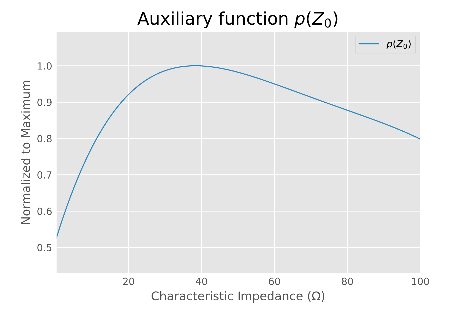 Image of the normalized auxiliary
function p
Image of the normalized auxiliary
function p
It resembles the classic problem of how maximum transmission power in a coaxial cable varies with impedance, reaching its maximum at Z0=38.5Ω. Therefore, the authors named it the “power” function.
p=d0+d1z0+d2z02+d3z03+d4z04pmax=kDout2P=ppmax
Where:
- d0=0.52, d1=0.0325, d2=−7.495⋅10−4, d3=6.854⋅10−6, d4=−2.331⋅10−8
- k=17.3875 (Note: Originally reported as 1.73875 in the paper, believed to be a typo)
The final high-frequency correction formula is:
C(f)=Cstatic(1−Pf2)−0.5
Where:
- f is frequency, in Gigahertz (GHz).
- P is the auxiliary “power” function.
For Z0∈[30,70], overall error is less than 2%; for Z0∈[10,100], overall error is less than 5%.
Code and Examples
Code: See Code 1: Chramiec-Piotrowski Empirical Formula Calculation.
Example: For an ideal vacuum line (3.5 mm/1.52 mm), capacitance is 39.75 fF (DC-1 GHz); notably, by keeping conductor diameters constant and “extracting” the dielectric to calculate the characteristic impedance of the “equivalent vacuum line,” the author found the vacuum data also applies to PTFE: for an ideal PTFE coaxial line (4.13/1.25 mm), the capacitance calculated by this method is 31.44-31.45 fF (DC-1 GHz), close to the Gajda-Stuchly model.
Appendix 5: Calculation of Short-Circuited Coaxial Line Parasitic Inductance
The author’s review of existing literature found methods for calculating the short-circuit impedance of coaxial transmission lines by Kennerh H. Wong (published 1992) and Chihyun Cho (published 2019). The calculation methods differ, but the results are highly consistent.
Besides the above methods, the methods in the following two papers are suspected to be incorrect and should not be used: D. C. X. Ung’s 2023 paper [57] cites Wong’s result, but the surface impedance formula in this paper is missing a 1/2, suspected to be a typo; the formula in Kang et al.’s 2005 paper [58] is similar to Cho et al.’s later formula but uses the coaxial cable impedance instead of the free space impedance, resulting in significant differences from the Wong and Cho formulas. Notably, Kang is also a co-author of Cho’s new paper, so Cho’s work can be seen as an improvement on the former.
Wong’s Formula
In 1992, Kennerh H. Wong, an engineer from HP’s microwave measurement division, proposed the impedance of a coaxial short (reference plane at the short) at a conference. As this report is official HP work, its credibility is high.
The calculation formula is as follows:
Zshort=(1+j)ωμσ12πln(Dd).
Where:
- j is the imaginary unit.
- ω=2πf is the angular frequency.
- σ and μ are the absolute conductivity and permeability of the shorting metal conductor.
- D and d are the outer and inner diameters of the cable.
Cho’s Formula
In 2019, Cho et al. from the Korea Research Institute of Standards and Science used a different short-circuit calculation formula in [20] (errata [21]) for calibrating 1.0 mm RF connections at 110 GHz. In this formula, the coaxial short problem is treated as the reflection of electromagnetic waves in free space. This is official work from the Korean national metrology lab, and its results have been verified by HFSS and cross-lab comparisons with NIST, also highly credible.
The calculation formulas are as follows:
Γshort=ηsurf−η0ηsurf+η0ηsurf=(1+j)ωμ2σ
Where:
- j is the imaginary unit.
- ω=2πf is the angular frequency.
- σ and μ are the absolute conductivity and permeability of the shorting metal conductor.
- η0 is the impedance of free space.
- ηsurf is the surface impedance of the shorting conductor.
Code and Examples
Code: See Code 2: Wong and Cho Short-Circuit Impedance Calculation.
Example: For a non-ferromagnetic (μ=μ0) ideal 3.5 mm/1.52 mm air coaxial line, even assuming very high loss in the shorting conductor σ=3.0⋅106 S/m, the phase shift at 110 GHz is only about 0.1 degrees. This shows that the phase shift of the short standard is mainly introduced by the pin/socket tolerances of the connector, not by the short itself. Furthermore, the figure below shows that Cho et al.’s formula differs only slightly from Wong’s formula.
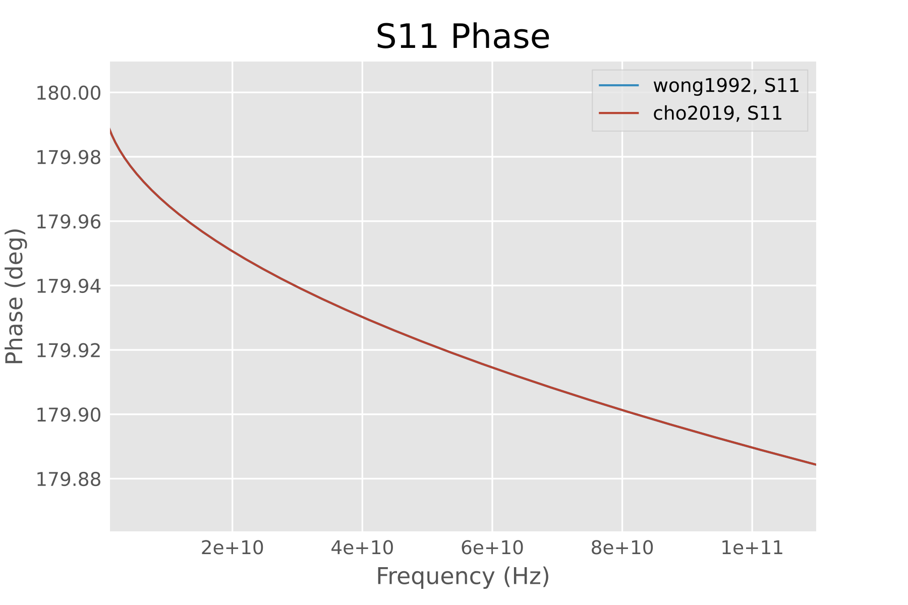 Comparison of calculation results from
Wong and Cho formulas
Comparison of calculation results from
Wong and Cho formulas
Code 0: Calkit Parameter Generation
The following Python script uses the scikit-rf library to compute the corresponding calkit S-parameters from their definitions.
import sys import numpy as np import skrf from skrf.media import DefinedGammaZ0 def keysight_calkit_offset_line(freq, offset_delay, offset_loss, offset_z0, port_z0): if offset_delay or offset_loss: alpha_l = (offset_loss * offset_delay) / (2 * offset_z0) alpha_l *= np.sqrt(freq.f / 1e9) beta_l = 2 * np.pi * freq.f * offset_delay + alpha_l zc = offset_z0 + (1 - 1j) * (offset_loss / (4 * np.pi * freq.f)) * np.sqrt(freq.f / 1e9) gamma_l = alpha_l + beta_l * 1j medium = DefinedGammaZ0(frequency=freq, z0_port=offset_z0, z0=zc, gamma=gamma_l) offset_line = medium.line(d=1, unit='m') return medium, offset_line else: medium = DefinedGammaZ0(frequency=freq, z0=offset_z0) line = medium.line(d=0) return medium, line def keysight_calkit_open(freq, offset_delay, offset_loss, c0, c1, c2, c3, offset_z0=50, port_z0=50): medium, line = keysight_calkit_offset_line(freq, offset_delay, offset_loss, offset_z0, port_z0) # Capacitance is defined with respect to the port impedance offset_z0, not the lossy # line impedance. In scikit-rf, the return values of `shunt_capacitor()` and `medium.open()` # methods are (correctly) referenced to the port impedance. if c0 or c1 or c2 or c3: poly = np.poly1d([c3, c2, c1, c0]) capacitance = medium.shunt_capacitor(poly(freq.f)) ** medium.open() else: capacitance = medium.open() return line ** capacitance def keysight_calkit_short(freq, offset_delay, offset_loss, l0, l1, l2, l3, offset_z0=50, port_z0=50): # Inductance is defined with respect to the port impedance offset_z0, not the lossy # line impedance. In scikit-rf, the return values of `inductor()` and `medium.short()` # methods are (correctly) referenced to the port impedance. medium, line = keysight_calkit_offset_line(freq, offset_delay, offset_loss, offset_z0, port_z0) if l0 or l1 or l2 or l3: poly = np.poly1d([l3, l2, l1, l0]) inductance = medium.inductor(poly(freq.f)) ** medium.short() else: inductance = medium.short() return line ** inductance def keysight_calkit_load(freq, offset_delay=0, offset_loss=0, offset_z0=50, port_z0=50): medium, line = keysight_calkit_offset_line(freq, offset_delay, offset_loss, offset_z0, port_z0) load = medium.match() return line ** load def plot_and_write(network): fig, ax = plt.subplots(1, 2) fig.set_size_inches(12, 5) network.plot_s_db(m=0, n=0, ax=ax[0], title="S11 Magnitude") network.plot_s_deg_unwrap(m=0, n=0, ax=ax[1], title="S11 Phase") filename = network.name.replace("/", "|") network.write_touchstone(filename) plt.savefig(filename + '.svg') if not "--no-plot" in sys.argv: plt.show() if __name__ == "__main__": from matplotlib import pyplot as plt skrf.stylely() freq = skrf.Frequency(1, 9000, 1001, "MHz") calkit_defs = [ { "name": "Keysight 85033E Pin", "open": { "offset_z0": 50, "offset_delay": 29.2e-12, "offset_loss": 2.2e9, "c0": 49.433e-15, "c1": -310.130e-27, "c2": 23.168e-36, "c3": -0.15966e-45, }, "short": { "offset_z0": 50, "offset_delay": 31.80e-12, "offset_loss": 2.36e9, "l0": 2.0765e-12, "l1": -108.5400e-24, "l2": 2.1705e-33, "l3": -0.0100e-42, }, }, { "name": "Keysight 85032F Pin", "open": { "offset_z0": 50, "offset_delay": 4.0856e-11, "offset_loss": 0.9300e9, "c0": 89.939e-15, "c1": 2536.800e-27, "c2": -264.990e-36, "c3": 13.400e-45 }, "short": { "offset_z0": 49.992, "offset_delay": 4.5955e-11, "offset_loss": 1.0870e9, "l0": 3.3998e-12, "l1": -496.4808e-24, "l2": 34.8314e-33, "l3": -0.7847e-42, }, }, { "name": "Keysight 85054D Pin", "open": { "offset_z0": 50, "offset_delay": 5.7993e-11, "offset_loss": 0.93e9, "c0": 89.9390e-15, "c1": 2536.7999e-27, "c2": -264.9901e-36, "c3": 13.400e-45 }, "short": { "offset_z0": 50, "offset_delay": 6.3078e-11, "offset_loss": 1.1273e9, "l0": 0.7563e-12, "l1": 459.8799e-24, "l2": -52.4290e-33, "l3": 1.5846e-42, }, }, { "name": "Keysight 85032BE Pin", "short": { "offset_z0": 50.209, "offset_delay": 1.7817e-11, "offset_loss": 2.1002e9, "l0": 0, "l1": 0, "l2": 0, "l3": 0, }, }, ] for calkit in calkit_defs: for termination in ["open", "short"]: if termination not in calkit.keys(): continue if termination == "open": std = keysight_calkit_open( freq, **calkit["open"] ) std.name = "%s %s" % (calkit["name"], "Open") elif termination == "short": std = keysight_calkit_short( freq, **calkit["short"] ) std.name = "%s %s" % (calkit["name"], "Short") else: raise KeyError("Unknown termination type: %s" % termination) plot_and_write(std)Code 1: Chramiec-Piotrowski Empirical Formula Calculation
The following Python script is a full implementation of the Chramiec-Piotrowski empirical formula.
from numpy import pi, log from scipy.constants import physical_constants def vacuum_coax_z0(d_outer, d_inner): """ Calculate the characteristic impedance of a coax cable in vacuum. """ z0_vacuum = physical_constants["characteristic impedance of vacuum"][0] return z0_vacuum * log(d_outer / d_inner) * (1 / (2 * pi)) def c_open_static_chramiec(d_outer, d_inner): """ The frequency-independent capacitance of a coax open circuit. For use at low-frequency only. At high-frequency, this solution requires a frequency-dependent correction, see c(). Maximum error is less than 1% (10-70 Ω z0), or 2.5% (10-70 Ω z0). Fitted by Chramiec-Piotrowski (eq. 6) [Chramiec1999] based on the numerical data from Somlo's theoretical solution [Somlo1967]. To obtain a well-defined open circuit, the outer coax conductor should be slightly extended out of the reference plane. It forms a circular waveguide below its cutoff frequency, suppressing radiation and parasitic environmental coupling if sufficiently long. Some Open standards for Vector Network Analyzers (VNAs) are designed this way, but many are not! Be sure your Open standard has no delay or transmission line inside (known as "offset open"). To be rigorous, the outer body must be extended - a dummy dust cap may be too short. [Chramiec1999] J. Chramiec and J. K. Piotrowski, "Universal formula for frequency-dependent coaxial open-end effect", Electronics Letters, vol. 35, pp. 1474–1475, 1999, doi: 10.1049/el:19990978. [Somlo1967] P. I. Somlo, "The Computation of Coaxial Line Step Capacitances," in IEEE Transactions on Microwave Theory and Techniques, vol. 15, no. 1, pp. 48-53, January 1967, doi: 10.1109/TMTT.1967.1126368. """ # Fringe capacitance of open-ended coax cables is the electric energy # stored in the vacuum outside the cable, so the dielectric material # of the coax cable itself can be neglected, only the inner and outer # conductor diameters matter. By removing the dielectric from a coax # cable and calculating the equivalent vacuum coax, fringe capacitance # can be found. z0 = vacuum_coax_z0(d_outer, d_inner) alpha = 2669.26 beta = 0.095 gamma = 5.95 delta = 14.72 epsilon = 4.7467 zeta = 1.102696e6 eta = 130.9 return ( ( (alpha * d_outer * z0 ** beta) / (gamma + log(delta * z0 ** epsilon + zeta)) ) - (eta * d_outer) ) * 1e-12 def c_open_chramiec(freq_list, d_outer, d_inner): """ The frequency-dependent capacitance of a coax open circuit. Maximum average error is less than 2% (30-70 Ω z0), or 5% (10-100 Ω z0). The frequency-independent term is fitted by Chramiec-Piotrowski using the numerical values from Somlo's earlier analytical solution, the frequency - dependent terms are fitted from the CAD model in Chramiec-Piotrowski's own papers. Note that the value 1.73875 in Eq. 5 is incorrect, it should be 17.3875, the former value is inconsistent with Fig. 2 of the paper, and inconsistent with Eq. 1 in [Chramiec2000] by the same authors, the computed factor is off by 10. The same typo is also corrected by Фатеев in a PhD thesis, see Eq. 2.5 in [Фатеев2023]. To obtain a well-defined open circuit, the outer coax conductor should be slightly extended out of the reference plane. It forms a circular waveguide below its cutoff frequency, suppressing radiation and parasitic environmental coupling if sufficiently long. Some Open standards for Vector Network Analyzers (VNAs) are designed this way, but many are not! Be sure your Open standard has no delay or transmission line inside (known as "offset open"). To be rigorous, the outer body must be extended - many generic Open standards use a dummy dust cap, which may be too short. [Somlo1967] P. I. Somlo, "The Computation of Coaxial Line Step Capacitances," in IEEE Transactions on Microwave Theory and Techniques, vol. 15, no. 1, pp. 48-53, January 1967, doi: 10.1109/TMTT.1967.1126368. [Chramiec1999] J. Chramiec and J. K. Piotrowski, "Universal formula for frequency-dependent coaxial open-end effect", Electronics Letters, vol. 35, pp. 1474–1475, 1999, doi: 10.1049/el:19990978. [Chramiec2000] J. Chramiec and M. Kitlinski, "Characterization of vector network analyzer coaxial calibration components," 13th International Conference on Microwaves, Radar and Wireless Communications. MIKON - 2000. Conference Proceedings (IEEE Cat. No.00EX428), Wroclaw, Poland, 2000, pp. 543-546 vol.2, doi: 10.1109/MIKON.2000.913991. [Фатеев2023] A.B. Фатеев, МЕТОДИКА ИЗМЕРЕНИЯ И КОНТРОЛЯ ЭЛЕКТРОФИЗИЧЕСКИХ ПАРАМЕТРОВ КОАКСИАЛЬНЫХ ИЗОЛЯТОРОВ В РАСШИРЕННОМ ТЕМПЕРАТУРНОМ ДИАПАЗОНЕ. https://postgraduate.tusur.ru/system/file_copies/files/000/003/737/original/Диссертация_Коренев_финал.pdf """ def p(d_outer, z0): """ Auxiliary function p (eq. 4). When p is normalized to its maximum value p_max, curiously the shape of the plot looks similar to the maximum transmitted power of a coax cable of a given characteristics impedance, its maxima is at z0 = 38.5 Ω. Thus this function is named p (for "power"). This function is almost independent of the value of d_outer """ # Normalization factor p_max (eq. 5), note that the value 1.73875 # in the original formula is incorrect! k = 17.3875 p_max = k * d_outer ** 2 # normalized auxiliary function p (eq. 4) d0 = 0.52 d1 = 0.0325 d2 = -7.495e-4 d3 = 6.854e-6 d4 = -2.331e-8 p = d0 + d1 * z0 + d2 * z0 ** 2 + d3 * z0 ** 3 + d4 * z0 ** 4 # return an actual value before normalization return p * p_max # Fringe capacitance of open-ended coax cables is the electric energy # stored in the vacuum outside the cable, so the dielectric material # of the coax cable itself can be neglected, only the inner and outer # conductor diameters matter. By removing the dielectric from a coax # cable and calculating the equivalent vacuum coax, fringe capacitance # can be found. z0 = vacuum_coax_z0(d_outer, d_inner) f_ghz = freq_list / 1e9 return c_open_static_chramiec(d_outer, d_inner) * (1 - p(d_outer, z0) * f_ghz ** 2) ** (-0.5) if __name__ == "__main__": print("3.5/1.52 mm coax: %.2f fF (DC), %.2f fF (1 GHz)" % ( c_open_static_chramiec(3.5e-3, 1.52e-3) * 1e15, c_open_chramiec(1e9, 3.5e-3, 1.52e-3) * 1e15 )) print("4.13/1.25 mm coax: %.2f fF (DC), %.2f fF (1 GHz)" % ( c_open_static_chramiec(4.13e-3, 1.25e-3) * 1e15, c_open_chramiec(1e9, 4.13e-3, 1.25e-3) * 1e15 ))Code 2: Wong and Cho Short-Circuit Impedance Calculation
from numpy import pi, sqrt, log from scipy.constants import mu_0, physical_constants from matplotlib import pyplot as plt import skrf skrf.stylely() # [Wong1992] K. H. Wong, “Characterization of calibration standards by # physical measurements,” in 39th ARFTG Conference Digest, vol. 21, # 1992, pp. 53–62. Official work by Hewlett-Packard's Microwave Technology # Division def short_wong1992(freq_list, d_outer, d_inner, mu_r, sigma): mu = mu_0 * mu_r omega = 2 * pi * freq_list scale_factor = (1 / (2 * pi)) * log(d_outer / d_inner) r_surf = sqrt(omega * mu_0 / (2 * sigma)) z_surf = (1 + 1j) * r_surf z_shorting_plane = z_surf * scale_factor return skrf.Network.from_z(frequency=freq, z=z_shorting_plane, name='wong1992') # [Cho2019] Chihyun Cho, Jin-Seob Kang, Joo-Gwang Lee, Hyunji Koo, # "Characterization of a 1 mm (DC to 110 GHz) calibration kit for VNA," # Journal of Electromagnetic Engineering and Science, vol. 19, no. 4, # pp. 272–278, 2019. # # [ChoErratum2021] Chihyun Cho, Jin-Seob Kang, Joo-Gwang Lee, Hyunji Koo, # "Erratum to 'Characterization of a 1 mm (DC to 110 GHz) Calibration Kit # for VNA'". Journal of Electromagnetic Engineering and Science. vol. 21. # pp. 165-165, 2021. # # Similar to [Wong1992], except that no scale factor is used for the # coax cables. Instead, the short circuit reflection in coax is approximated # as the EM wave reflection from a piece of metal. # # Note that this paper also contains a typo for the offset transmission # line equation, See [ChoErratum2021]. def short_cho2019(freq_list, d_outer, d_inner, mu_r, sigma): mu = mu_0 * mu_r omega = 2 * pi * freq_list r_surf = sqrt(omega * mu / (2 * sigma)) z_surf = (1 + 1j) * r_surf # approximate coax reflection using free space reflection z_freespace = physical_constants["characteristic impedance of vacuum"][0] z_shorting_plane = z_surf s_shorting_plane = (z_shorting_plane - z_freespace) / (z_shorting_plane + z_freespace) # reference impedance is still 50 ohms return skrf.Network(frequency=freq, s=s_shorting_plane, name='cho2019') def plot_mag_phase(network_list, m=0, n=0): for network in network_list: network.plot_s_mag(m=0, n=0, title="S11 Magnitude") plt.show() for network in network_list: network.plot_s_db(m=0, n=0, title="S11 dB") plt.show() plt.ticklabel_format(useOffset=False, style='plain') for network in network_list: network.plot_s_deg(m=0, n=0, title="S11 Phase") plt.show() if __name__ == "__main__": input_kwargs = { "mu_r": 1, "sigma": 3.0e6, "d_outer": 3.5, "d_inner": 1.52 } freq = skrf.Frequency(1e9, 110e9, 1001, unit='Hz') plot_mag_phase([ short_wong1992(freq.f, **input_kwargs), short_cho2019(freq.f, **input_kwargs) ])Code 3: Numerical Simulation of Incorrect Calibration
import argparse import numpy as np from scipy.optimize import curve_fit import skrf from skrf.media import DefinedGammaZ0 import matplotlib.pyplot as plt skrf.stylely() def build_parser(): parser = argparse.ArgumentParser() parser.add_argument('--plot', action="store_true", dest="plot", default=True) parser.add_argument('--no-plot', action="store_false", dest="plot") parser.add_argument('--output-imgs', type=str, default=[], nargs='+') return parser def sol(cal_def_list, cal_meas_list, dut_raw): """ Apply One-Port SOL calibration to correct dut_raw data. * cal_def_list: Three skrf.networks that define the ideal, perfect S-parameters of the standards, in the order of Open, Short, Load. * cal_meas_list: Three skrf.networks that carry the measured imperfect S-parameters of the same standards, in the order of Open, Short, Load. * dut_raw: One skrf.networks that carries the measured imperfect DUT S-parameters. * Return: One skrf.networks that carries the measured DUT S-parameters after correction. """ assert len(cal_def_list) == len(cal_meas_list) == 3 algo = skrf.calibration.OnePort( measured=cal_meas_list, ideals=cal_def_list ) algo.run() dut_corrected = algo.apply_cal(dut_raw) return dut_corrected def measure(f, c, l): frequency = skrf.Frequency.from_f(f, unit='Hz') c *= 1e-15 l *= 1e-12 ideal_medium = DefinedGammaZ0(frequency) calkit_ideal = [ ideal_medium.short(), ideal_medium.open(), ideal_medium.match() ] calkit_hp85033e = [ skrf.Network("output/Keysight 85033E Pin Short.s1p"), skrf.Network("output/Keysight 85033E Pin Open.s1p"), ideal_medium.match() ] calkit_unknown = [ ideal_medium.inductor(L=l) ** ideal_medium.short(), ideal_medium.shunt_capacitor(C=c) ** ideal_medium.open(), ideal_medium.match() ] # perform a wrong calibration using Keysight offset delay calkit, # but with flush standard definition, then we measure the cheap # unknown calkit measurement = [ sol(calkit_ideal, calkit_hp85033e, calkit_unknown[0]), sol(calkit_ideal, calkit_hp85033e, calkit_unknown[1]) ] return measurement def f_measure(f, c, l): measurement = measure(f[0:len(f)//2], c, l) return ( np.concatenate([ measurement[1].s_deg_unwrap[:,0,0], measurement[0].s_deg_unwrap[:,0,0], ]) ) if __name__ == "__main__": parser = build_parser() args = parser.parse_args() calkit_unknown_measured = [ skrf.Network("output/Vendor SMA Short.s1p"), skrf.Network("output/Vendor SMA Open.s1p"), ] frequency = calkit_unknown_measured[0].frequency x = np.concatenate([frequency.f, frequency.f]) y = np.concatenate([ calkit_unknown_measured[1].s_deg_unwrap[:,0,0], calkit_unknown_measured[0].s_deg_unwrap[:,0,0], ]) popt, pcov = curve_fit( f_measure, x, y, bounds=([0, 0], [100, 100]) ) print("C = %s fF\nL = %s pH" % (popt[0], popt[1])) measurement = measure(frequency.f, popt[0], popt[1]) measurement[0].name = "Fitted (%.2f pH)" % popt[1] measurement[1].name = "Fitted (%.2f fF)" % popt[0] for i in range(2): plt.figure() calkit_unknown_measured[i].plot_s_deg_unwrap() measurement[i].plot_s_deg_unwrap() if args.plot: plt.show() if args.output_imgs: plt.savefig(args.output_imgs[i]) ideal_medium = DefinedGammaZ0(frequency) fitted = [ ideal_medium.inductor(L=popt[1] * 1e-12) ** ideal_medium.short(), ideal_medium.shunt_capacitor(C=popt[0] * 1e-15) ** ideal_medium.open() ] fitted[0].name = "Fitted (%.2f pH)" % popt[1] fitted[1].name = "Fitted (%.2f fF)" % popt[0] for i in range(2): plt.figure() fitted[i].plot_s_deg_unwrap() if args.plot: plt.show() if args.output_imgs: plt.savefig(args.output_imgs[i + 2])Bibliography
- [1] “市售网络仪校准件开路器和短路器相位误差有多大?,” 波络科技,
Weixin Official Accounts Platform, Jan. 2018. Available:
https://mp.weixin.qq.com/s/TQd7vAtnRxkEfzM714ULjQ
- [2] C. Whisky, “Scattering parameters of a two-port network (a
bandpass filter).” Apr. 2020. Available:
https://commons.wikimedia.org/wiki/File:Parametri_S.jpg
- [3] J. Hillairet and A. Arsenovic, “Measuring a multiport device
with a 2-port network analyzer,” scikit-rf, Software Documentation,
2021.
- [4] “IEEE standard for electrical characterization of printed
circuit board and related interconnects at frequencies up to 50 GHz,”
IEEE, IEEE Std P370, Jan. 2021. doi:
10.1109/IEEESTD.2021.9316329.
- [5] J. Chramiec and J. K. Piotrowski, “Universal formula for
frequency-dependent coaxial open-end effect,” Electronics Letters,
vol. 35, no. 17, pp. 1474–1475, 1999, doi:
10.1049/el:19990978.
- [6] J. R. Whinnery and H. W. Jamieson, “Equivalent circuits for
discontinuities in transmission lines,” Proceedings of the IRE, vol.
32, no. 2, pp. 98–114, Feb. 1944, doi:
10.1109/JRPROC.1944.229737.
- [7] J. R. Whinnery, H. W. Jamieson, and T. E. Robbins, “Coaxial-line
discontinuities,” Proceedings of the IRE, vol. 32, no. 11, pp.
695–709, Nov. 1944, doi:
10.1109/JRPROC.1944.234027.
- [8] N. Marcuvitz, Ed., Waveguide handbook, First Edition. in
Massachusetts Institute of Technology Radiation Laboratory Series,
no. 10. New York: McGraw-Hill, 1951. Available:
https://archive.org/details/MITRadiationLaboratorySeries10WaveguideHandbook
- [9] P. I. Somlo, “The computation of coaxial line step
capacitances,” IEEE Transactions on Microwave Theory and Techniques,
vol. 15, no. 1, pp. 48–53, Jan. 1967, doi:
10.1109/TMTT.1967.1126368.
- [10] P. I. Somlo, “The discontinuity capacitance and the effective
position of a shielded open circuit in a coaxial line,” Proceedings
of the Institution of Radio and Electrical Engineers Australia, vol.
28, no. 1, pp. 7–9, Jan. 1967, doi:
10.5281/zenodo.17015632.
- [11] M. Razaz and J. B. Davies, “Capacitance of the abrupt
transition from coaxial-to-circular waveguide,” IEEE Transactions on
Microwave Theory and Techniques, vol. 27, no. 6, pp. 564–569, Jun.
1979, doi:
10.1109/TMTT.1979.1129672.
- [12] E. Costamagna and A. Fanni, “Computing capacitances via the
Schwarz-Christoffel transformation in structures with rotational
symmetry,” IEEE Transactions on Magnetics, vol. 34, no. 5, pp.
2497–2500, Sep. 1998, doi:
10.1109/20.717575.
- [13] G. B. Gajda and S. S. Stuchly, “Numerical analysis of
open-ended coaxial lines,” IEEE Transactions on Microwave Theory and
Techniques, vol. 31, no. 5, pp. 380–384, May 1983, doi:
10.1109/TMTT.1983.1131507.
- [14] A. P. Gregory, T. E. Hodgetts, R. N. Clarke, and G. J. Hill,
“Calculations of the fringing capacitance of cylindrical electrodes,”
National Physical Laboratory, Electromagnetic Technologies Group,
Electromagnetic and Electrochemical Technologies Department, NPL
Report TQE 28, Nov. 2023. doi:
10.47120/npl.TQE28.
- [15] T. E. Hodgetts, “The calculation of the equivalent circuits of
coaxial-line step discontinuities,” Royal Signals; Radar
Establishment, RSRE Memorandum RSRE-MEMO-3422, 1981. Available:
https://apps.dtic.mil/sti/html/tr/ADA111962/
- [16] “IEEE standard for precision coaxial connectors (DC to 110
GHz),” IEEE, IEEE Std 287, 2007. doi:
10.1109/IEEESTD.2007.4317507.
- [17] “Radio-frequency connectors – part 15: Sectional specification
– RF coaxial connectors with inner diameter of outer conductor 4,13 mm
(0,163 in) with threaded coupling – characteristic impedance 50
$\mathrm{\Omega}$ (type SMA),” International Electrotechnical
Commission, International Standard IEC 61169-15:2021, 2021. Available:
https://web.archive.org/web/20250522235025/https://cdn4.booksdl.lc/get.php?md5=b5eed07a644a9ccefc1ac06baa2cc46a&key=K3JPYWD98VPB60P6
- [18] TubeTimeUS, “Cross section of an SMA mated pair.” Apr. 2019.
Available:
https://commons.wikimedia.org/wiki/File:Cross_section_of_an_SMA_mated_pair.png
- [19] K. H. Wong, “Characterization of calibration standards by
physical measurements,” in 39th ARFTG Conference Digest, Jun. 1992,
pp. 53–62. doi:
10.1109/ARFTG.1992.326972.
- [20] C. Cho, J.-S. Kang, J.-G. Lee, and H. Koo, “Characterization of
a 1 mm (DC to 110 GHz) Calibration Kit for VNA,” J. Electromagn. Eng.
Sci, vol. 19, no. 4, pp. 272–278, 2019, doi:
10.26866/jees.2019.19.4.272.
- [21] C. Cho, J.-S. Kang, J.-G. Lee, and H. Koo, “Erratum to
‘Characterization of a 1 mm (DC to 110 GHz) calibration kit for VNA’,”
J. Electromagn. Eng. Sci, vol. 21, no. 2, pp. 165–165, 2021, doi:
10.26866/jees.2021.21.2.e.
- [22] “Keysight Vector Network Analyzer Calibration Kit Standards
Definitions,” Keysight Technologies, 2024. Available:
https://web.archive.org/web/20250828172137/https://www.keysight.com/us/en/assets/9922-01521/technical-specifications/Calibration-Kit-Definitions.pdf
- [23] K. Poulsen, “How to fabricate a N male and female calibration
kit with arbitrary calibration data for VNWA 2 and VNWA3.” Feb. 2014.
Available:
https://www.hamcom.dk/VNWA/How%20to%20fabricate%20a%20N%20Male%20and%20Female%20calibration%20kit.pdf
- [24]
“网络分析仪在完成开路/短路/负载校准后直接测试开路器和短路器,在smith圆图上会得到一个点吗?,”
波络科技, Weixin Official Accounts Platform, Jan. 2018. Available:
https://mp.weixin.qq.com/s/P3axtjV3eOiPAvwvHXhIog
- [25] “矢量网络分析仪校准件开路器背后的秘密,” 波络科技, Weixin
Official Accounts Platform, Sep. 2023. Available:
https://mp.weixin.qq.com/s/gngxAw1V0Nr5tUBBu50I2A
- [26] Boonuo(淘宝店铺), “6-26.5GHz
网络分析仪SMA/3.5mm校准套件含开短路器/负载(淘宝商品:547147324755).”
Available:
https://web.archive.org/web/20250913211501/https://img.alicdn.com/imgextra/i1/49139067/O1CN011B9vp42GqkDRtXN8H_!!49139067.jpg
- [27] SGLabs, “HP Agilent Keysight 11866A Calibration kit APC 7 mm
OSL.” Accessed: Sep. 14, 2025. [Online]. Available:
https://web.archive.org/web/20250913203409/http://www.sglabs.it/public/SgLabs_m_HP%20Agilent%2011866A_4.jpg
- [28] “HP 11866A APC-7 calibration kit,” Hewlett-Packard, Operating
and Service Manual 11866-90003, Dec. 1977. Available:
https://web.archive.org/web/20250913204122/https://eadn-wc01-3361420.nxedge.io/cdn/wp-content/uploads/pdf/A_11866A.pdf
- [29] eRecycler Online, “Agilent HP 85032-60011 Open Short 50-ohm
Type N calibration kit.” Jun. 2025. Available:
https://web.archive.org/web/20250913225144/https://erecycleronline.com/product/agilent-hp-85032-60011-open-short-50ohm-type-n-calibration-kit/
- [30] “Agilent Technologies 85032B/E 50 Ω Type-N calibration kits,”
Agilent Technologies, User’s and Service Guide 85032-90020, Aug. 2010.
Available:
https://web.archive.org/web/20250913230837/https://www.artisantg.com/info/Agilent_85032B_Manual.pdf
- [31] B. Bianco, A. Corana, L. Gogioso, S. Ridella, and M. Parodi,
“Open-circuited coaxial lines as standards for microwave
measurements,” Electronics Letters, vol. 16, no. 10, pp. 373–374,
1980, doi:
10.1049/el:19800265.
- [32] Boonuo(淘宝店铺), “3/6/8.5/9/14/18/20GHz
SMA校准件网分天分NanoVNA 三/五件套(淘宝商品:536798357382).”
Available:
https://web.archive.org/web/20250913214208/https://img.alicdn.com/imgextra/i2/49139067/O1CN0130SaeD2Gqk4qCKBPY_!!49139067.jpg
- [33] 波络科技, “深圳市波络科技有限公司.” Apr. 2022. Available:
http://www.szwavenet.com/
- [34] T. Baier, “VNWA help file,” Software Documentation, May 2023.
Available:
https://web.archive.org/web/20250911085648/https://www.sdr-kits.net/documents/VNWA_HELP.pdf
- [35] “HP 85033C 3.5 mm calibration kit,” Hewlett-Packard, Operating
and Service Manual 85033-90007, May 1990. Available:
https://web.archive.org/web/20250911170632/https://www.rlscientific.com/documenti/HP85033C.pdf
- [36] “Keysight technologies DCA probes & accessories,” Keysight
Technologies, Technical Overview 5991-2340EN, Aug. 2014. Available:
https://web.archive.org/web/20250911163504/https://prc.keysight.com/Content/PDF_Files/5991-2340EN.pdf
- [37] “1011-01-SA2 转接器,” 北京维创时通科技有限公司, 产品规格书,
Dec. 2019. Available:
https://web.archive.org/web/20250911163858/http://www.witctech.com/media/converter/1011-01-SA2.pdf
- [38] “SMA-JKG 转接器,” 北京东方旭普科技有限公司, 产品规格书,
Feb. 2024. Available:
https://web.archive.org/web/20250911164826/https://img.alicdn.com/imgextra/i2/849838761/O1CN01lCB1382Eaaxy4v1Oa_!!849838761.png
- [39] “4021-01-SA1 转接器,” 北京维创时通科技有限公司, 产品规格书,
Jun. 2020. Available:
https://web.archive.org/web/20250911165503/http://www.witctech.com/media/converter/4021-01-SA1.pdf
- [40] K. Poulsen, “How to select the very best parts for a SMA
calibration kit for the DG8SAQ VNWA.” Nov. 2013. Available:
http://www.hamcom.dk/VNWA/How%20to%20select%20the%20very%20best%20parts%20for%20a%20SMA%20calibration%20kit%20for%20the%20DG8SAQ%20VNWA.pdf
- [41] P. I. Somlo and J. D. Hunter, Microwave impedance
measurement. in IEE Electrical measurement series, no. 2. Stevenage:
Peregrinus, 1985. Available:
https://archive.org/details/microwaveimpedan0000soml
- [42] D. Rytting, “Network analyzer error models and calibration
methods,” Agilent Technologies, 2005. Available:
https://web.archive.org/web/20250606052055/http://emlab.uiuc.edu/ece451/appnotes/Rytting_NAModels.pdf
- [43] D. M. Pozar, Microwave engineering, Fourth edition. Hoboken,
NJ: John Wiley & Sons, Inc, 2012.
- [44] “SOLT calibration standards creation,” scikit-rf, Project
Documentation, 2025. Available:
https://scikit-rf.readthedocs.io/en/latest/examples/metrology/SOLT%20Calibration%20Standards%20Creation.html
- [45] “Specifying calibration standards and kits for Agilent vector
network analyzers,” Agilent Technologies, Application Note 1287-11,
Aug. 2009. Available:
https://web.archive.org/web/20230605182500/https://people.ece.ubc.ca/robertor/Links_files/Files/AN-1287-11.pdf
- [46] D. C. DeGroot, K. L. Reed, and J. A. Jargon, “Equivalent
circuit models for coaxial OSLT standards,” in 54th ARFTG Conference
Digest, Dec. 2000, pp. 1–13. doi:
10.1109/ARFTG.1999.327370.
- [47] M. Wollensack and J. Hoffmann, “METAS VNA Tools - Math
Reference V2.9.0.” Federal Institute of Metrology (METAS), Aug. 2025.
Available:
https://web.archive.org/web/20250829054357/https://www.metas.ch/dam/metas/en/data/fachbereiche/hochfrequenz/vna-tools/vnatools_v2_9_0/vnatools_math_v2.9.0-e.pdf.download.pdf/vnatools_math_v2.9.0-e.pdf
- [48] J. P. Grant, R. N. Clarke, G. T. Symm, and N. M. Spyrou, “A
critical study of the open-ended coaxial line sensor technique for RF
and microwave complex permittivity measurements,” Journal of Physics
E: Scientific Instruments, vol. 22, no. 9, p. 757, Sep. 1989, doi:
10.1088/0022-3735/22/9/015.
- [49] T. lchino, H. Ohkawara, and N. Sugihara, “Vector impedance
analysis to 1000 MHz,” Hewlett-Packard Journal, vol. 31, no. 1, p.
32, Jan. 1980, Available:
https://web.archive.org/web/20240619220328/https://hparchive.com/Journals/HPJ-1980-01.pdf
- [50] N. M. Ridler, “Connectors, air lines and RF impedance,” in
14th IEE Microwave Measurements Training Course, 2005, pp. 9/1–9/18.
doi: 10.1049/ic:20050150.
- [51] C. A. Hoer, “Some questions and answers concerning air lines as
impedance standards,” in 29th ARFTG Conference Digest, Jun. 1987,
pp. 161–173. doi:
10.1109/ARFTG.1987.323862.
- [52] R. D. Pollard, “Compensation technique improves measurements
for a range of mechanically compatible connectors,” Microwave
Journal, vol. 37, no. 10, p. 91+, Oct. 1994, Accessed: Aug. 07, 2025.
[Online]. Available:
https://web.archive.org/web/20250807132508/https://file.elecfans.com/web1/M00/61/D5/o4YBAFuGjPGAAB2WABS0KM2eFts501.pdf
- [53] J. P. Hoffmann, P. Leuchtman, J. Ruefenacht, and K. Wong,
“S-parameters of slotted and slotless coaxial connectors,” in 2009
74th ARFTG Microwave Measurement Conference, Nov. 2009, pp. 1–5. doi:
10.1109/ARFTG74.2009.5439109.
- [54] J. Ruefenacht and J. Hoffmann, “Coaxial connector effects,”
Torino, May 2011. doi:
10.13140/2.1.3666.7685.
- [55] K. Wong and J. Hoffmann, “Improving VNA measurement accuracy by
including connector effects in the models of calibration standards,”
in 82nd ARFTG Microwave Measurement Conference, Nov. 2013, pp. 1–7.
doi:
10.1109/ARFTG-2.2013.6737334.
- [56] D. Woods, “Shielded-open-circuit discontinuity capacitance of a
coaxial line,” Proceedings of the Institution of Electrical
Engineers, vol. 119, no. 12, pp. 1691–1692, 1972, doi:
10.1049/piee.1972.0338.
- [57] D. C. X. Ung, “Modelling coaxial SHORT and OPEN calibration
standards,” in 2023 5th Australian Microwave Symposium (AMS), Feb.
2023, pp. 49–50. doi:
10.1109/AMS57822.2023.10062343.
- [58] J.-S. Kang, J.-H. Kim, and D.-C. Kim, “Phase analysis of
coaxial short and open circuits,” IEEE Transactions on
Instrumentation and Measurement, vol. 54, no. 2, pp. 701–704, Apr.
2005, doi:
10.1109/TIM.2004.843335.


