Quantum neural networks form Gaussian processes

Neural networks (NNs) have revolutionized machine learning (ML) and artificial intelligence. Their tremendous success across many fields of research in a wide variety of applications^1,2,3 is certainly astonishing. Although much of this success has come from heuristics, the past few decades have witnessed a notable increase in our theoretical understanding of their inner workings. One of the most interesting results regarding NNs is that fully connected models with a single hidden layer converge to Gaussian processes (GPs) in the limit of a large number of hidden neurons when the parameters are initialized from independent and identically distributed (i.i.d.) priors⁴. More recently, it has been shown that i.i.d.-initialized, fully connected, multi-layer NNs also converge to GPs in the infinite-width limit⁵. Furthermore, other architectures, such as convolutional NNs⁶, transformers⁷ and recurrent NNs⁸, are also GPs under certain assumptions. More than just a mathematical curiosity, the correspondence between NNs and GPs has opened up the possibility of performing exact Bayesian inference for regression and learning tasks using wide NNs^4,9. Training wide NNs with GPs requires inverting the covariance matrix of the training set, a process that can be computationally expensive. Recent studies have explored the use of quantum linear algebraic techniques to efficiently perform these matrix inversions, potentially offering polynomial speed-ups over standard classical methods^10,11.

Indeed, the advent of quantum computers has stimulated enormous interest in merging quantum computing with ML, leading to the thriving field of quantum machine learning (QML)^{12,13,14,15,16}. Rapid progress has been made in this field, largely fuelled by the hope that QML may provide a quantum advantage in the near term for some practically relevant problems. Although the prospects for such a practical quantum advantage remain unclear¹⁷, there are several promising analytical results^18,19,20,21. Still, much remains to be learned about QML models.

In this work, we contribute to the QML body of knowledge by proving that under certain conditions the outputs of deep quantum neural networks (QNNs)—parametrized quantum circuits acting on input states drawn from a training set—converge to GPs in the limit of large Hilbert space dimension (Fig. 1). Our results are derived for QNNs that are Haar random over the unitary and orthogonal groups. Unlike the classical case, where the proof of the emergence of GPs stems from the central limit theorem, the situation becomes more intricate in the quantum setting as the entries of the QNN are not independent. Namely, the rows and columns of a unitary matrix are constrained to be mutually orthonormal. Hence, our proof strategy boils down to showing that each moment of the output distribution of a QNN converges to that of a multivariate Gaussian. Importantly, we also show that the Bayesian distribution of a QNN acting on qubits is efficient (inefficient) for predicting local (global) measurements. We then use our results to provide a precise characterization of the concentration of measure phenomenon in deep random quantum circuits^{22,23,24,25,26,27}. Our theorems indicate that the expectation values, as well as the gradients, of Haar-random processes concentrate faster than previously reported²⁸. Finally, we discuss how our results can be leveraged to study QNNs that are not fully Haar random but instead form t-designs, which constitutes a much more practical assumption^29,30,31.

Fig. 1: Schematic of our main results.

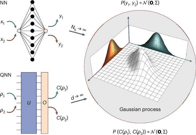
It is well known that certain classical NNs with N_h neurons per hidden layer become GPs when N_h → ∞. That is, given inputs x₁ and x₂, and corresponding outputs y₁ and y₂, then the joint probability P(y₁, y₂) is a multivariate Gaussian \({\mathcal{N}}({\bf{0}},\varSigma)\). In this work, we show that a similar result holds under certain conditions for deep QNNs in the limit of large Hilbert space dimension, d → ∞. Now, given quantum states ρ₁ and ρ₂, \(C(\rho )={\rm{Tr}}[U\rho {U}^{\dagger }O]\) is such that \(P(C({\rho }_{1}),C({\rho }_{2}))={\mathcal{N}}({\bf{0}},\varSigma)\).

We begin by introducing GPs.

Definition 1

A collection of random variables {X₁, X₂, …} is a GP if and only if, for every finite set of indices {1, 2, …, m}, the vector (X₁, X₂, …, X_m) follows a multivariate Gaussian distribution, which we denote as \({\mathcal{N}}({{\mu }},{\varSigma})\). Said otherwise, every linear combination of {X₁, X₂, …, X_m} follows a univariate Gaussian distribution.

In particular, \({\mathcal{N}}({{\mu }},\varSigma)\) is determined by its m-dimensional mean vector \({\mathbf{\upmu }}=({\mathbb{E}}[{X}_{1}],\ldots ,{\mathbb{E}}[{X}_{m}])\), where \(\mathbb{E}\) denotes the expectation value, and by its m × m-dimensional covariance matrix with entries (Σ)_αβ = Cov[X_α, X_β].

GPs are extremely important in ML because they can be used as a form of kernel method to solve learning tasks^4,9. For instance, consider a regression problem where the data domain is \({\mathscr{X}}={\mathbb{R}}\) and the label domain is \({\mathscr{Y}}={\mathbb{R}}\). Instead of finding a single function \(f:{\mathscr{X}}\to {\mathscr{Y}}\) that solves the regression task, a GP assigns probabilities to a set of possible f(x), such that the probabilities are higher for the ‘more likely’ functions. Following a Bayesian inference approach, one then selects the functions that best agree with some set of empirical observations^9,16.

Under this framework, the output over the distribution of functions f(x), for \(x\in {\mathscr{X}}\), is a random variable. Then, given a set of training samples x₁, …, x_m and some covariance function \(\kappa (x,{x}^{{\prime} })\), Definition 1 implies that if one has a GP, the outputs f(x₁), …, f(x_m) are random variables sampled from some multivariate Gaussian distribution \({\mathcal{N}}({{\mu }},\varSigma)\). From here, the GP is used to make predictions about the output f(x_m+1) (for some new data instance x_m+1), given the previous observations f(x₁), …, f(x_m). Explicitly, one constructs the joint distribution P(f(x₁), …, f(x_m), f(x_m+1)) from the averages and the covariance function κ to obtain the sought-after ‘predictive distribution’ P(f(x_m+1) ∣ f(x₁), …, f(x_m)) through marginalization. The power of the GP relies on this distribution usually containing less uncertainty than \(P(f({x}_{m+1}))={\mathcal{N}}({\mathbb{E}}[f({x}_{m+1})],\kappa ({x}_{m+1},{x}_{m+1}))\) (Methods).

In the following we consider a setting where one is given repeated access to a dataset \({\mathscr{D}}\) containing quantum states \({\{{\rho }_{i}\}}_{i}\) on a d-dimensional Hilbert space that satisfy \({\rm{Tr}}[{\rho }_{i}^{2}]\in \varOmega ({1}/{{\rm{poly}}(\log (d))})\) for all i. We will make no assumptions regarding the origin of these states, as they can correspond to classical data encoded in quantum states^32,33 or quantum data obtained from some quantum mechanical process^34,35. Then, the states are sent through a deep QNN, denoted U. Although in general U can be parametrized by some set of trainable parameters θ, we leave this dependence implicit for ease of notation. At the output of the circuit, one measures the expectation value of a traceless Hermitian operator taken from a set \({\mathscr{O}}={\{{O}_{j}\}}_{j}\) such that Tr[O_jO_j′] = dδ_j,j′ and \({O}_{j}^{2}={\mathbb{1}}\), for all j and j′ (for example, Pauli strings). We denote the QNN outputs as

Then, we collect these quantities over some set of states from \({\mathscr{D}}\) and some set of measurements from \({\mathscr{O}}\) in a vector

As we will show below, in the large-d limit, \({\mathscr{C}}\) converges to a GP when the QNN unitaries U are sampled according to the Haar measure on \({\mathbb{U}}(d\,)\) and \({\mathbb{O}}(d\,)\), the degree-d unitary and orthogonal groups, respectively (Fig. 1). Recall that \({\mathbb{U}}(d)=\{U\in {{\mathbb{C}}}^{d\times d},U{U}^{\dagger }={U}^{\dagger }U={\mathbb{1}}\}\) and that \({\mathbb{O}}(d)=\{U\in {{\mathbb{R}}}^{d\times d},U{U}^\mathrm{T}={U}^\mathrm{T}U={\mathbb{1}}\}\). We will henceforth use the notation \({{\mathbb{E}}}_{{\mathbb{U}}(d)}\) and \({{\mathbb{E}}}_{{\mathbb{O}}(d)}\) to, respectively, denote Haar averages over \({\mathbb{U}}(d)\) and \({\mathbb{O}}(d)\). Moreover, we assume that when the circuit is sampled from \({\mathbb{O}}(d)\), the states in \({\mathscr{D}}\) and the measurement operators in \({\mathscr{O}}\) are real valued.

Moment computation in the large-d limit

As we discuss in Methods, we cannot rely on simple arguments based on the central limit theorem to show that \({\mathscr{C}}\) forms a GP. Hence, our proof strategy is based on computing all the moments of the vector \({\mathscr{C}}\) and showing that they asymptotically match those of a multivariate Gaussian distribution. To conclude the proof we show that these moments unequivocally determine the distribution, for which we can use Carleman’s condition^36,37. We refer the reader to the Supplementary Information for the detailed proofs of the results in this manuscript.

First, we present the following lemma.

Lemma 1

Let C_j(ρ_i) be the expectation value of a Haar-random QNN as in equation (1). Then for any \({\rho }_{i}\in {\mathscr{D}}\) and \({O}_{j}\in{\mathscr{O}}\),

Moreover, for any pair of states \({\rho }_{i},{\rho }_{{i}^{{\prime} }}\in {\mathscr{D}}\) and operators \({O}_{j},{O}_{{j}^{{\prime} }}\in {\mathscr{O}}\), we have

if \(j\ne {j}^{{\prime} }\) and

if \(j={j}^{{\prime} }\). Here, we have defined \(\varSigma_{i,{i}^{{\prime} }}^{G}={\operatorname{Cov}}_{G}[{C}_{j}(\,{\rho }_{i}){C}_{j}(\,{\rho }_{{i}^{{\prime} }})]\), where \(G={\mathbb{U}}(d),{\mathbb{O}}(d)\).

Lemma 1 shows that the expectation value of the QNN outputs is always zero. More notably, it indicates that the covariance between the outputs is null if we measure different observables (even if we use the same input state and the same circuit). This implies that the distributions C_j(ρ_i) and C_j′(ρ_i′) are uncorrelated if j ≠ j′. That is, knowledge of the measurement outcomes for one observable and different input states does not provide any information about the outcomes of other measurements, at these or any other input states. Therefore, we will focus in the following on when \({\mathscr{C}}\) contains expectation values for different states but the same operator. In this case, Lemma 1 shows that the covariances will be positive, zero or negative depending on whether Tr[ρ_iρ_i′] is larger, equal to or smaller than 1/d, respectively.

We now state a useful result.

Lemma 2

Let \({\mathscr{C}}\) be a vector of expectation values of a Haar-random QNN as in equation (2), where one measures the same operator O_j over a set of states from \({\mathscr{D}}\). Furthermore, let \({\rho }_{{i}_{1}},\ldots ,{\rho }_{{i}_{k}}\in {\mathscr{D}}\) be a multiset of states taken from those in \({\mathscr{C}}\). In the large-d limit, if k is odd, then \({{\mathbb{E}}}_{{\mathbb{U}}(d)}\left[{C}_{j}(\,{\rho }_{{i}_{1}})\cdots {C}_{j}(\,{\rho }_{{i}_{k}})\right]={{\mathbb{E}}}_{{\mathbb{O}}(d)}\left[{C}_{j}(\,{\rho }_{{i}_{1}})\cdots {C}_{j}(\,{\rho }_{{i}_{k}})\right]=0\). Moreover, if k is even and \(\operatorname{Tr}[{\rho }_{i}{\rho }_{{i}^{{\prime} }}]\in \varOmega ({1}/{{\rm{poly}}(\log (d))})\) for all i and i′, we have

where the summation runs over all the possible disjoint pairing of indices in the set {1, 2, …, k}, T_k, and the product is over the different pairs in each pairing.

Using Lemma 2 as our main tool, we will be able to prove that deep QNNs form GPs for different types of datasets. Table 1 summarizes our main results.

Positively correlated GPs

We begin by studying the case when the states in the dataset satisfy Tr[ρ_iρ_i′] ∈ Ω(1/poly(log(d))) for all \({\rho }_{i},{\rho }_{{i}^{{\prime} }}\in {\mathscr{D}}\). According to Lemma 1, this implies that the variables are positively correlated. In the large-d limit, we can derive the following theorem.

Theorem 1

Under the same conditions for which Lemma 2 holds, the vector \({\mathscr{C}}\) forms a GP with mean vector μ = 0 and covariance matrix given by \(\varSigma_{i,{i}^{{\prime} }}^{{\mathbb{U}}}=\frac{\varSigma_{i,{i}^{{\prime} }}^{{\mathbb{O}}}}{2}=\frac{\operatorname{Tr}[\,{\rho }_{i}{\rho }_{{i}^{{\prime} }}]}{d}\).

Theorem 1 indicates that the covariances for the orthogonal group are twice as large as those arising from the unitary group. Figure 2 presents results obtained by numerically simulating a unitary Haar-random QNN for a system of n = 18 qubits. The circuits were sampled using known results for the distribution of the entries of random unitary matrices³⁶. In the left panels of Fig. 2, we show the corresponding two-dimensional GP obtained for two initial states that satisfy Tr[ρ_iρ_i′] ∈ Ω(1). We can see that the variables are positively correlated in accordance with the prediction in Theorem 1.

Fig. 2: Two-dimensional GPs.

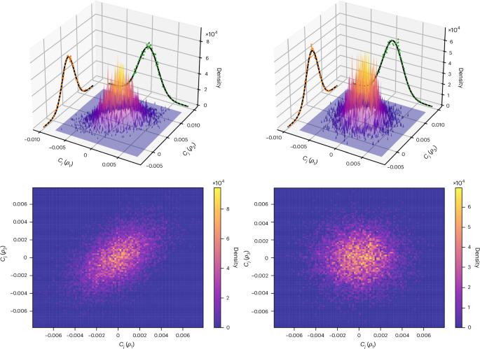
We plot the joint probability density function, as well as its scaled marginals, for the measurement outcomes at the output of a unitary Haar-random QNN acting on n = 18 qubits. The measured observable is O_j = Z₁, where Z₁ denotes the Pauli z operator on the first qubit. Moreover, the input states are for the left column, ρ₁ = |0〉 〈0|^⊗n and ρ₂ = |GHZ〉 〈GHZ| with \(\left\vert {\rm{GHZ}}\right\rangle =\frac{1}{\sqrt{2}}({\left\vert 0\right\rangle }^{\otimes n}+{\left\vert 1\right\rangle }^{\otimes n})\), and for the right column, ρ₁ and ρ₃ = |Ψ〉 〈Ψ| with \(\left\vert \varPsi \right\rangle =\frac{1}{\sqrt{d}}{\left\vert 0\right\rangle }^{\otimes n}+\sqrt{1-\frac{1}{d}}{\left\vert 1\right\rangle }^{\otimes n}\). In both cases we took 10⁴ samples.

Source data

That the outputs of deep QNNs form GPs reveals a deep connection between QNNs and quantum kernel methods. Although it has already been pointed out that QNN-based QML constitutes a form of kernel-based learning³⁸, our results solidify this connection for Haar-random circuits. Notably, we can recognize that the kernel arising in the GP covariance matrix is proportional to the fidelity kernel, that is, to the Hilbert–Schmidt inner product between the data states^38,39,40. Moreover, because the predictive distribution of a GP can be expressed as a function of the covariance matrix (Methods) and, thus, of the kernel entries, our results further cement that quantum models such as those in equation (1) are functions in the reproducing kernel Hilbert space³⁸.

Uncorrelated GPs

We now consider the case when Tr[ρ_iρ_i′] = 1/d for all \({\rho }_{i}\ne {\rho }_{{i}^{{\prime} }}\in {\mathscr{D}}\). We found the following result.

Theorem 2

Let \({\mathscr{C}}\) be a vector of expectation values of an operator in \({\mathscr{O}}\) over a set of states from \({\mathscr{D}}\), as in equation (2). If Tr[ρ_iρ_i′] = 1/d for all i ≠ i′, then in the large-d limit, \({\mathscr{C}}\) forms a GP with mean vector μ = 0 and diagonal covariance matrix

In the right panel of Fig. 2, we plot the GP corresponding to two initial states such that Tr[ρ_iρ_i′] = 1/d. In this case, the variables seem to be uncorrelated, as predicted by Theorem 2. Importantly, in Supplementary Section C.3, we show that when Tr[ρ_iρ_i′] ∈ o(1/poly(log(d))) for all ρ_i ≠ ρ_i′, \({\mathscr{C}}\) will form an uncorrelated GP if one takes the covariance matrix to be approximately diagonal in the large-d limit. Then, in Methods we show that the results of Theorems 1 and 2 are valid for generalized datasets, where the conditions on the overlaps need be met only on average.

Negatively correlated GPs

Here we study orthogonal states, that is when Tr[ρ_iρ_i′] = 0 for all \({\rho }_{i}\ne {\rho }_{{i}^{{\prime} }}\in {\mathscr{D}}\). We prove the following theorem.

Theorem 3

Let \({\mathscr{C}}\) be a vector of expectation values of an operator in \({\mathscr{O}}\) over a set of states from \({\mathscr{D}}\), as in equation (2). If Tr[ρ_iρ_i′] = 0 for all i ≠ i′, then in the large-d limit, \({\mathscr{C}}\) forms a GP with mean vector μ = 0 and covariance matrix

Note that the magnitude of the covariances is Θ(1/d²) whereas that of the variances is Θ(1/d poly(log(d))). That is, in the large-d limit, the covariances are much smaller than the variances.

Deep QNN outcomes and their linear combination

In this section and the following ones we will study the implications of Theorems 1, 2 and 3. Unless stated otherwise, the corollaries we present can be applied to all considered datasets (Table 1).

First, we study the univariate probability distribution P(C_j(ρ_i)).

Corollary 1

Let C_j(ρ_i) be the expectation value of a Haar-random QNN as in equation (1). Then, for any \({\rho }_{i}\in {\mathscr{D}}\) and \({O}_{j}\in {\mathscr{O}}\), we have

where σ² = 1/d or 2/d when U is Haar random over \({\mathbb{U}}(d)\) and \({\mathbb{O}}(d)\), respectively.

Corollary 1 shows that when a single state from \({\mathscr{D}}\) is sent through the QNN and a single operator from \({\mathscr{O}}\) is measured, the outcomes follow a Gaussian distribution with a variance that vanishes inversely proportional to the Hilbert space dimension. This means that for large problem sizes, we can expect the results to be extremely concentrated around their mean (see below for more details). Figure 3 compares the predictions from Corollary 1 to numerical simulations. The simulations match our theoretical results very closely, for both the unitary and the orthogonal groups. Moreover, the standard deviation for orthogonal Haar-random QNNs is larger than that for unitary ones. In Fig. 3 we also plot the quotient \({{\mathbb{E}}[{C}_{j}{(\,{\rho }_{i})}^{k}]}/{{\mathbb{E}}{[{C}_{j}{(\,{\rho }_{i})}^{2}]}^{k/2}}\) obtained from our numerics, and we verify that it follows the value \(\frac{k!}{{2}^{k/2}(k/2)!}\) for a Gaussian distribution.

Fig. 3: Probability density function for C_j(ρ_i) for Haar-random QNNs and different problem sizes.

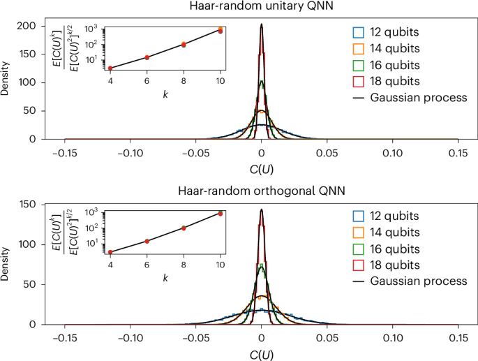
We consider unitary and orthogonal QNNs with n qubits, and we take ρ_i = |0〉 〈0|^⊗n and O_j = Z₁. The coloured histograms are built from 10⁴ samples in each case. The solid black lines represent the corresponding Gaussian distributions \({\mathcal{N}}\left(0,{\sigma }^{2}\right)\), where σ² is given in Corollary 1. The insets show the numerical versus predicted value of \({\mathbb{E}}[{C}_{j}{({\rho }_{i})}^{k}]/{\mathbb{E}}{[{C}_{j}{({\rho }_{i})}^{2}]}^{k/2}\). For a Gaussian distribution with zero mean, the quotient is \(\frac{k!}{{2}^{k/2}(k/2)!}\) (solid black line).

Source data

At this point, it is worth making an important remark. According to Definition 1, if \({\mathscr{C}}\) forms a GP, then any linear combination of its entries will follow a univariate Gaussian distribution. In particular, if \(\{{C}_{j}(\,{\rho }_{1}),{C}_{j}(\,{\rho }_{2}),\ldots ,{C}_{j}(\,{\rho }_{m})\}\subseteq {\mathscr{C}}\), then \(P({C}_{j}(\,\widetilde{\rho }))\) with \(\widetilde{\rho }=\mathop{\sum }\nolimits_{i = 1}^{m}{c}_{i}{\rho }_{i}\) will be equal to \({\mathcal{N}}(0,{\widetilde{\sigma }}^{2})\) for some \(\widetilde{\sigma }\). Note that the real-valued coefficients \({\{{c}_{i}\}}_{i = 1}^{m}\) need not be a probability distribution, meaning that \(\widetilde{\rho }\) is not necessarily a quantum state. This then raises an important question: What happens if \(\widetilde{\rho }\propto {\mathbb{1}}\)? A direct calculation shows that \({C}_{j}(\,\widetilde{\rho })=\mathop{\sum }\nolimits_{i = 1}^{m}{C}_{j}({c}_{i}{\rho }_{i})\propto {\rm{Tr}}[U{\mathbb{1}}{U}^{\,\dagger }{O}_{j}]={\rm{Tr}}[{O}_{j}]=0\). How can we then unify these two perspectives? On the one hand, \({C}_{j}(\,\widetilde{\rho })\) should be normally distributed, but, on the other hand, we know that it is always constant. To solve this issue, note that the only dataset we considered for which the identity can be constructed is the one where Tr[ρ_iρ_i′] = 0 for all i ≠ i′ (this follows because if \({\mathscr{D}}\) contains a complete basis, then for any \(\widetilde{\rho }\in {{\mathscr{D}}}^{\perp }\), one has that if \({\rm{Tr}}[\widetilde{\rho }{\rho }_{i}]=0\) for all \({\rho }_{i}\in {\mathscr{D}}\), then \(\widetilde{\rho }=0\); here, \({{\mathscr{D}}}^{\perp }\) denotes the kernel of the projector onto the subspace spanned by the vectors in \({\mathscr{D}}\)). In that case, we can leverage Theorem 3 along with the identity \({\widetilde{\sigma}}^{2}=\operatorname{Var}_{G}\left[\sum_{i = 1}^{d}{C}_{j}(\,{\rho }_{i})\right]=\sum_{i,{i}^{{\prime} }}\operatorname{Cov}_{G}[{C}_{j}(\,{\rho }_{i}),{C}_{j}(\,{\rho }_{{i}^{{\prime} }})]\) to explicitly prove that \(\operatorname{Var}_{G}\left[\sum_{i = 1}^{d}{C}_{j}(\,{\rho }_{i})\right]=0\) (for \(G={\mathbb{U}}(d),{\mathbb{O}}(d)\)). Hence, we find a zero-variance Gaussian distribution, that is, a delta distribution for the outcomes of the QNN (as expected).

Predictive power of the GP for qubit systems

Consider that we are given a (potentially continuous) set \({\mathcal{D}}\) of n-qubit states and the following task, divided into two phases. In a first data-acquisition phase, one is allowed to send some states from \({\mathcal{D}}\) through some fixed unknown unitary V acting on n′ ≤ n qubits, perform measurements and record the outcomes. Crucially, the unitary V need not be Haar random but could be, in principle, any unitary (even the identity). Then, during a second prediction phase, access to V is no longer granted, but one has to predict the value of Tr[Vρ_iV^†O] for any \({\rho }_{i}\in {\mathcal{D}}\), where O is some fixed Pauli string acting on the n′ qubits.

Although one could opt for some tomographic approach to learn V and solve the previous task, our work enables us to use the predictive power of the GP. In particular, one starts with the prior that V could be any unitary in \({\mathbb{U}}({2}^{{n}^{{\prime} }})\). Thus, the probability distribution of Tr[Vρ_iV^†O] is a univariate Gaussian as per our main theorems (assuming \({\mathcal{D}}\) satisfies the appropriate conditions). In the first stage, one measures the expectation value Tr[Vρ_iV^†O] for some training set \({\mathscr{D}}\subset {\mathcal{D}}\). Then, during the second stage, one computes the overlaps between the states in \({\mathscr{D}}\) (to build the covariance matrix) as well as with any new state from \({\mathcal{D}}\) on which we wish to apply the predictive power of the GP. These measurements can then be used to update the prior and make predictions (see Methods for the details of this procedure).

As evidenced from Lemma 1, the entries of the covariance matrix are suppressed as 2^n′, that is, exponentially in n′. Hence, and as explained in Methods, this implies that if V acts on all n qubits (or on Θ(n) qubits), then an exponential number of measurements will be needed if we are to use Bayesian inference to learn any information about new outcomes given previous ones. However, the situation becomes much more favourable if the QNN acts on \({n}^{{\prime} }\in {\mathcal{O}}(\log (n))\) qubits, as here only a polynomial number of measurements are needed to use the predictive power of the GP (provided that the overlaps between the n′-qubit quantum states are not super-polynomially vanishing in n). In fact, we show in Fig. 4 simulations on up to n = 200 qubits where a GP is used as a regression tool to interpolate or extrapolate and accurately predict measurement results at the output of a quantum dynamical process (see Methods for details).

Fig. 4: Quantum GP regression.

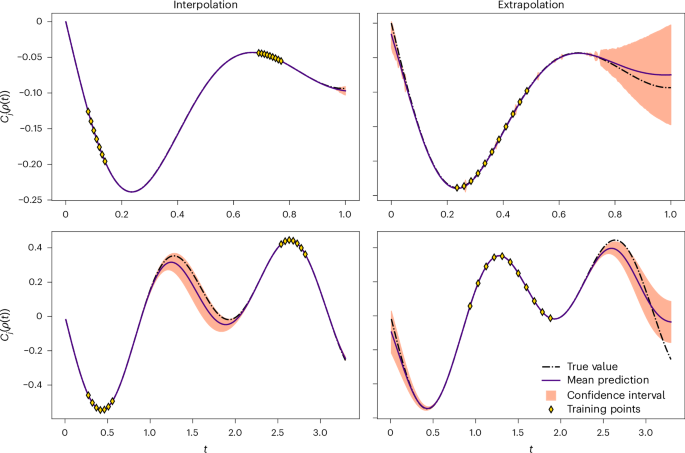
The plots show the time evolution of two local random Pauli operators of an n-qubit system under an XY Hamiltonian with random transverse fields in one (bottom panels, n = 200) and two spatial dimensions (top panels, n = 25). Details can be found in Methods. The dots are observations from which the predictions were inferred. The latter correspond to the solid purple line (mean). The shaded regions indicate a two-sigma (~95%) confidence interval. We also plot the true value (black line) for reference.

Source data

Concentration of measure

In this section, we show that Corollary 1 provides a more precise characterization of the concentration of measure and the barren-plateau phenomena for Haar-random circuits than that found in the literature^{22,23,24,25,26,27,28}. First, it implies that deep orthogonal QNNs will exhibit barren plateaux, a result not previously known. Second, we recall that in standard analyses of barren plateaux, one looks only at the first two moments of the distribution of cost values C_j(ρ_i) (or, similarly, of gradient values ∂_θC_j(ρ_i)). Then one uses Chebyshev’s inequality, which states that for any c > 0, the probability P(|X| ≥ c) ≤ Var[X]/c², to prove that P(∣C_j(ρ_i)∣ ≥ c) and P(∣∂_θC_j(ρ_i)∣ ≥ c) are in \({\mathcal{O}}({1}/{d})\) (refs. ^23,27). However, having a full characterization of P(C_j(ρ_i)) allows us to compute tail probabilities and obtain a much tighter bound. For instance, as U is Haar random over \({\mathbb{U}}(d)\), the following corollary holds.

Corollary 2

Let C_j(ρ_i) be the expectation value of a Haar random QNN as in equation (1). Assuming that there exists a parametrized gate in U of the form e^−iθH for some Pauli operator H, then

Corollary 2 indicates that the QNN outputs and their gradients actually concentrate with a probability that vanishes exponentially with d. In an n-qubit system where d = 2ⁿ, then P(∣C_j(ρ_i)∣ ≥ c) and P(∣∂_θC_j(ρ_i)∣ ≥ c) are doubly exponentially vanishing with n. The tightness of our bound arises because Chebyshev’s inequality is loose for highly narrow Gaussian distributions. Moreover, our bound is also tighter than that provided by Levi’s lemma²⁸, as it includes an extra \({\mathcal{O}}({1}/{\sqrt{d}})\) factor. Corollary 2 also implies that the narrow gorge region of the landscape²⁷, that is, the fraction of non-concentrated C_j(ρ_i) values, also decreases exponentially with d.

Furthermore, we show in Methods how our results can be used to study the concentration of functions of QNN outcomes, for example, standard loss functions used in the literature, like the mean-squared error.

Implications for t-designs

We now note that our results allow us to characterize the output distribution for QNNs that form t-designs, that is, for QNNs whose unitary distributions have the same properties up to the first t moments as sampling random unitaries from \({\mathbb{U}}(d)\) with respect to the Haar measure. With this in mind, one can readily see that the following corollary holds.

Corollary 3

Let U be drawn from a t-design. Then, under the same conditions for which Theorems 1, 2 and 3hold, the vector \({\mathscr{C}}\) matches the first t moments of a GP.

Corollary 3 extends our results beyond the strict condition of the QNN being Haar random to being a t-design, which is a more realistic assumption^29,30,31. In particular, we can study the concentration phenomenon in t-designs. Using an extension of Chebyshev’s inequality to higher-order moments leads to \(P(| {C}_{j}(\,{\rho }_{i})| \ge c),\) \(P(| {\partial }_{\theta }{C}_{j}(\,{\rho }_{i})| \ge c)\in {\mathcal{O}}\scriptstyle\left(\scriptstyle\frac{\left(2\left\lfloor \frac{t}{2}\right\rfloor \right)!}{{2}^{\left\lfloor \scriptstyle\frac{t}{2}\right\rfloor }{(d{c}^{2})}^{\left\lfloor \scriptstyle\frac{t}{2}\right\rfloor }\left(\left\lfloor \scriptstyle\frac{t}{2}\right\rfloor \right)!}\right)\) (see Supplementary Section M for a proof). Note that for t = 2, we recover the known concentration result for barren plateaux, but for t ≥ 4, we obtain new polynomial-in-d-tighter bounds.

We have shown in this manuscript that under certain conditions, the output distribution of deep Haar-random QNNs converges to a GP in the limit of large Hilbert space dimension. Although this result had been conjectured in ref. ¹⁵, a formal proof was still lacking. We remark that although our result mirrors its classical counterpart, namely that certain classical NNs form GPs, there exist nuances that differentiate our findings from the classical case. For instance, we need to make assumptions on the states processed by the QNN as well as on the measurement operator. Moreover, some of these assumptions are unavoidable, as Haar-random QNNs will not necessarily always converge to a GP. That is, not all QNNs and all measurements will lead to a GP. As an example, if O_j is a projector onto a computational basis state, then one recovers a Porter–Thomas distribution⁴¹. Ultimately, these subtleties arise because the entries of unitary matrices are not independent. In contrast, classical NNs are not subject to this constraint.

Note that our theorems have further implications beyond those discussed here. First and foremost, that GPs can be efficiently used for regression in certain cases paves the way for new and exciting research avenues at the intersection of quantum information and Bayesian learning. Moreover, we envision that our methods and results will be useful in more general settings where Haar-random unitaries or t-designs are considered, such as quantum scramblers and black holes^26,42,43, many-body physics⁴⁴, quantum decouplers and quantum error correction⁴⁵. Finally, we leave for future work the study of whether GPs arise in other architectures, such as matchgate circuits^46,47.

Sketch of the proof of our main results

Because our main results are mostly based on Lemmas 1 and 2, we will here outline the main steps used to prove these lemmas. In particular, to prove them, we need to calculate, in the large-d limit, quantities of the form

for arbitrary k and for \(G={\mathbb{U}}(d),{\mathbb{O}}(d)\). Here, the operator Λ is defined as \(\varLambda ={\rho }_{{i}_{1}}\otimes \cdots \otimes {\rho }_{{i}_{k}}\), where the states ρ_i belong to \({\mathscr{D}}\) and where O is an operator in \({\mathscr{O}}\). The first moment μ (k = 1) and the second moments \(\varSigma_{i,{i}^{{\prime} }}^{G}\) (k = 2) can be directly computed using standard formulae for integration over the unitary and orthogonal groups (Supplementary Sections C and D). This readily recovers the results in Lemma 1. However, for larger k, a direct computation quickly becomes intractable, and we need to resort to asymptotic Weingarten calculations. More concretely, let us exemplify our calculations for the unitary group and for when the states in the dataset are such that Tr[ρ_iρ_i′] ∈ Ω(1/poly(log(d))) for all \({\rho }_{i},{\rho }_{{i}^{{\prime} }}\in {\mathscr{D}}\). As shown in Supplementary Section C.1, we can prove the following lemma.

Lemma 3

Let X be an operator in \({\mathcal{B}}({{\mathcal{H}}}^{\otimes k})\), the set of bounded linear operators acting on the k-fold tensor product of a d-dimensional Hilbert space \({\mathcal{H}}\). Let S_k be the symmetric group on k items, and let P_d be the subsystem permuting representation of S_k in \({{\mathcal{H}}}^{\otimes k}\). Then, for large Hilbert space dimension (d → ∞), the twirl of X over \({\mathbb{U}}(d)\) is

where the constants c_σ,π are in \({\mathcal{O}}(1/d)\).

Recall that the subsystem permuting representation of a permutation σ ∈ S_k is

Lemma 3 implies that equation (10) is equivalent to

Note that, by definition, because O is traceless and such that \({O}^{2}={\mathbb{1}}\), then Tr[P_d(σ)O^⊗k] = 0 for odd k (and for all σ). This result implies that all the odd moments are exactly zero, and also that the non-zero contributions in equation (12) for the even moments come from permutations consisting of cycles of even length. Note that as a direct consequence, the first moment \({{\mathbb{E}}}_{{\mathbb{U}}(d)}\left[{\rm{Tr}}[U{\rho }_{i}{U}^{\dagger }O]\right]\) is zero for any \({\rho }_{i}\in {\mathscr{D}}\), and, thus, we have μ = 0. To compute higher moments, we show that Tr[P_d(σ)O^⊗k] = d^r if k is even and σ is a product of r disjoint cycles of even length. The maximum of Tr[P_d(σ)O^⊗k] is, therefore, achieved when r is maximal, that is, when σ is a product of k/2 disjoint transpositions (cycles of length two), leading to Tr[P_d(σ)O^⊗k] = d^k/2. Then, we look at the factors Tr[ΛP_d(σ)] and include them in the analysis. We have that for all π and σ in S_k,

Moreover, because Tr[ρ_iρ_i′] ∈ Ω(1/poly(log(d))) for all pair of states \({\rho }_{i},{\rho }_{{i}^{{\prime} }}\in {\mathscr{D}}\), it holds that if σ is a product of k/2 disjoint transpositions, then

where the \({\widetilde{\varOmega}}\) notation omits poly(log(d))⁻¹ factors, whereas

for any other σ. Note that if σ consist only of transpositions, then it is its own inverse, that is, σ = σ⁻¹.

It immediately follows that for fixed k and d → ∞, the second sum in equation (12) is suppressed at least inversely proportional to the dimension of the Hilbert space with respect to the first one (that is, exponentially in the number of qubits for QNNs made out of qubits). Note that as long as k scales with d as \({\mathcal{O}}(\log \log d)\), our asymptotic analysis and, hence, the convergence to a GP are still valid. This can be seen because there are \(k!-\frac{k!}{{2}^{k/2}(k/2)!}\) permutations that are not the product of disjoint transpositions. Hence, we find

where we used Stirling’s approximation for the factorial and replaced k = log log d. As this ratio is quasi-polynomial in log d but all contributions that arise from permutations that are not the product of disjoint transpositions are suppressed as \({\mathcal{O}}({1}/{d})\), the conclusion follows.

Likewise, the contributions in the first sum in equation (12) coming from permutations that are not the product of k/2 disjoint transpositions are also suppressed at least inversely proportional to the Hilbert space dimension. Therefore, in the large-d limit, we arrive at

where we have defined T_k ⊆ S_k to be the subset of permutations that are exactly given by a product of k/2 disjoint transpositions. Note that this is precisely the statement in Lemma 2.

From here we can easily see that if every state in Λ is the same, that is, if \({\rho }_{{i}_{\lambda }}=\rho\) for λ = 1, …, k, then Tr[ρ_iρ_i′] = 1 for all t and t′, and we need to count how many terms there are in equation (16). Specifically, we need to count how many different ways there are to split k elements into pairs (with k even). A straightforward calculation shows that

Therefore, we arrive at

Identifying σ² = 1/d implies that the moments \({{\mathbb{E}}}_{{\mathbb{U}}(d)}[{\rm{Tr}}{\left[U\rho {U}^{\dagger }O\right]}^{k}]\) exactly match those of a Gaussian distribution \({\mathcal{N}}(0,{\sigma }^{2})\).

To prove that these moments unequivocally determine the distribution of \({\mathscr{C}}\), we use Carleman’s condition.

Lemma 4

(Carleman’s condition, Hamburger case³⁷). Let γ_k be the (finite) moments of the distribution of a random variable X that can take values on the real line \({\mathbb{R}}\). These moments determine uniquely the distribution of X if

Explicitly, we have

Hence, Carleman’s condition is satisfied according to Lemma 4, and P(C_j(ρ_i)) is distributed following a Gaussian distribution.

A similar argument can be given to show that the moments of \({\mathscr{C}}\) match those of a GP. Here, we need to compare equation (16) with the kth-order moments of a GP, which are provided by Isserlis’s theorem⁴⁸. Specifically, if we want to compute a kth-order moment of a GP, then we have that \({\mathbb{E}}[{X}_{1}{X}_{2}\cdots {X}_{k}]=0\) if k is odd, and

if k is even. Clearly, equation (16) matches equation (21) by identifying Cov[X_t, X_t′] = Tr[ρ_tρ_t′]/d. We can again prove that these moments uniquely determine the distribution of \({\mathscr{C}}\) because if its marginal distributions are determinate from Carleman’s condition (see above), then so is the distribution of \({\mathscr{C}}\) (ref. ³⁷). Hence, \({\mathscr{C}}\) forms a GP.

Generalized datasets

Up to this point we have derived our theorems by imposing strict conditions on the overlaps between every pair of states in the dataset. However, we can extend these results to when the conditions are met only on average when sampling states over \({\mathscr{D}}\).

Theorem 4

The results of Theorems 1and 2will hold, on average, if \({{\mathbb{E}}}_{{\rho }_{i},{\rho }_{{i}^{{\prime} }} \sim {\mathscr{D}}}\operatorname{Tr}[\,{\rho }_{i}{\rho }_{{i}^{{\prime} }}]\in \varOmega \left(\scriptstyle\frac{1}{{\rm{poly}}(\log (d))}\right)\) and \({{\mathbb{E}}}_{{\rho }_{i},{\rho }_{{i}^{{\prime} }} \sim {\mathscr{D}}}{\rm{Tr}}[\,{\rho }_{i}{\rho }_{{i}^{{\prime} }}]=\frac{1}{d}\), respectively.

In Theorem 4 we generalized the results of Theorems 1 and 2 to hold on average when (1) \({{\mathbb{E}}}_{{\rho }_{i},{\rho }_{{i}^{{\prime} }} \sim {\mathscr{D}}}\operatorname{Tr}[{\rho }_{i}{\rho }_{{i}^{{\prime} }}]\in \varOmega \left({1}/{{\rm{poly}}(\log (d))}\right)\) and (2) \({{\mathbb{E}}}_{{\rho }_{i},{\rho }_{{i}^{{\prime} }} \sim {\mathscr{D}}}\operatorname{Tr}[{\rho }_{i}{\rho }_{{i}^{{\prime} }}]={1}/{d}\), respectively. Interestingly, these two cases have practical relevance. Let us start with case (1). Consider a multiclass classification problem, where each state ρ_i in \({\mathscr{D}}\) belongs to one of Y classes, with \(Y\in {\mathcal{O}}(1)\), and where the dataset is composed of an (approximately) equal number of states from each class. That is, for each ρ_i we can assign a label y_i = 1, …, Y. Then, we assume that the classes are well separated in the Hilbert feature space, a standard and sufficient assumption for the model to be able to solve the learning task^32,35. By well separated, we mean that

In this case, it can be verified that for any pair of states ρ_i and ρ_i′ sampled from \({\mathscr{D}}\), one has \({{\mathbb{E}}}_{{\rho }_{i},{\rho }_{{i}^{{\prime} }} \sim {\mathscr{D}}}[\operatorname{Tr}[{\rho }_{i}{\rho }_{{i}^{{\prime} }}]]\in \varOmega \left({1}/{{\rm{poly}}(\log (d))}\right)\).

Next, let us evaluate case (2). This situation arises when the states in \({\mathscr{D}}\) are Haar-random states. Indeed, we can readily show that

In the first equality we used that sampling pure Haar-random states ρ_i and ρ_i′ from the Haar measure is equivalent to taking two reference pure states ρ₀ and ρ′₀ and evolving them with Haar-random unitaries. We used in the second equality the left-invariance of the Haar measure, and in the third equality, we explicitly performed the integration (Supplementary Section C).

Learning with the GP

In this section we will review the basic formalism for learning with GPs and then discuss conditions under which such learning is efficient.

Let C be a GP. Then, by definition, given a collection of inputs \({\{{x}_{i}\}}_{i = 1}^{m}\), C is determined by its m-dimensional mean vector μ, and its m × m-dimensional covariance matrix Σ. In the following, we will assume that the mean of C is zero and that the entries of its covariance matrix are expressed as κ(x_i, x_i′). That is,

This allows us to know that, a priori, the distribution of values for any f(x_i) will take the form

with \({\sigma }_{i}^{2}=\kappa ({x}_{i},{x}_{i})\).

Now, let us consider the task of using m observations, which we will collect in a vector y, to predict the value at x_m+1. First, if the observations are noiseless, then y = (y(x₁), …, y(x_m)) is equal to C = (C(x₁), …, C(x_m)). That is, C = y. Here, we can use that C forms a GP to find^9,49

where μ(C(x_m+1)) and σ²(C(x_m+1)), respectively, denote the mean and variance of the associated Gaussian probability distribution. These are given by

The vector m has entries m_i = κ(x_m+1, x_i). Comparing equations (25) and (26), we can see that using Bayesian statistics to obtain the predictive distribution of P(C(x_m+1)∣C) shifts the mean from zero to m^T ⋅ Σ⁻¹ ⋅ C. The variance is decreased from \({\sigma }_{m+1}^{2}\) by a quantity m^T ⋅ Σ⁻¹ ⋅ m. The decrease in variance follows because we are incorporating knowledge about the observations and, thus, decreasing the uncertainty.

From the above discussion, we can provide some intuition behind the differences between our three main theorems. From equation (28), it is clear that we can learn the most when the states in the dataset and the new state ρ_m+1 are similar (Theorem 1). Intuitively, this makes sense, as the more similar the training states are, the better we can predict the output through the QNN of a new state closely resembling the training set. One can readily verify that if one wishes to make predictions on a new state ρ_m+1 for which Tr[ρ_m+1ρ_i] = 1/d for all states ρ_i in the training set, then m = 0, meaning that we cannot update the prior (Theorem 2). This again makes perfect sense, as an overlap of 1/d is precisely the expected overlap between a Haar-random state and any other pure state. This result thus implies that we cannot use training data to make predictions on a Haar random ρ_m+1. Finally, the case of orthogonal states in Theorem 3 is fundamentally different from the uncorrelated one because two generic states are not expected to be orthogonal. Thus, we can still extract information as per equation (28).

In a realistic scenario, we would expect that noise will occur during our observation procedure. For simplicity, we model this noise as Gaussian noise, so that y(x_i) = C(x_i) + ε_i, where the noise terms ε_i are assumed to be independently drawn from the same distribution \(P({\varepsilon }_{i})={\mathcal{N}}(0,{\sigma }_{N}^{2})\). Now, because we have assumed that the noise is drawn independently, we know that the likelihood of obtaining a set of observations y given the model values C is given by \(P(\,{\boldsymbol{y}}| {\boldsymbol{C}}\,)={\mathcal{N}}({\boldsymbol{C}},{\sigma }_{N}^{2}{\mathbb{1}})\). In this case, we can find the probability distribution^9,49:

where now we have

We used in the first and the second equalities the explicit decomposition of the probability, along with Bayes and marginalization rules. We can see that the probability is still governed by a Gaussian distribution except that the inverse of Σ has been replaced by the inverse of \(\varSigma+{\sigma }_{N}^{2}{\mathbb{1}}\).

The previous results can be readily used to study whether learning with the GP will be efficient in the presence of finite sampling. First, let us assume that the QNN acts on all the qudits of the states in \({\mathscr{D}}\) and that we measure the same O_j at the output of the circuit. As such, the noise terms ε_i are taken to be drawn from the same distribution \(P({\varepsilon }_{i})={\mathcal{N}}(0,{\sigma }_{N}^{2})\) with \({\sigma }_{N}^{2}={1}/{N}\), and N the number of shots used to estimate each y(ρ_i). In this case, we can prove that the GP cannot be used to efficiently predict the outputs of the QNN from Bayesian statistics, as stated in the following theorem, whose proof can be found in Supplementary Section K.

Theorem 5

Consider a GP obtained from a Haar-random QNN. Given the set of observations (y(ρ₁), …, y(ρ_m)) obtained from \(N\in {\mathcal{O}}({\rm{poly}}(\log (d)))\) measurements, then the predictive distribution of the GP is trivial:

where σ² is given by Corollary 1.

Specifically, Theorem 5 shows that by spending only a poly-logarithmic-in-d (polynomial in n) number of measurements, one cannot use Bayesian statistical theory to learn any information about new outcomes given previous ones. The key insight behind Theorem 5 is that the covariance-matrix entries are suppressed as \({\mathcal{O}}({1}/{d})\) whereas the noise terms produce a statistical variance that is inversely proportional to the number of measurements. Hence, \(\varSigma+{\sigma }_{N}^{2}{\mathbb{1}}\approx {\sigma }_{N}^{2}{\mathbb{1}}\) in the large-d limit.

Next, for simplicity, let us focus on when the system has n qubits, so that the Hilbert space dimension is d = 2ⁿ (as in the main text). Moreover, we assume that the QNN and the measurement operator O_j act on m ≤ n qubits and that expectation values are again measured with \(N\in {\mathcal{O}}({\rm{poly}}(\log (d)))\) shots. When \(m\in {\mathcal{O}}(\log (n))\), Lemma 1 tells us that the covariance-matrix entries are suppressed only as Ω(1/poly(n)), provided that the overlaps on the reduced states on m qubits are in Ω(1/poly(n)). Because \({\sigma }_{N}^{2}=\frac{1}{N}\), it suffices to choose N polynomially large in n to attain \(\varSigma+{\sigma }_{N}^{2}{\mathbb{1}}\approx\varSigma\) in the large-d limit.

Details for the numerical simulations

We provide here the details of the numerical simulations demonstrating GP regression (Fig. 4). To create the dataset \({\mathcal{D}}\), we consider a quantum dynamical process in which an initial state ρ(0) is evolved under an XY Hamiltonian with local random transverse fields to produce the state ρ(t) at time t. Therefore, the states in \({\mathcal{D}}\) are states at arbitrary times, and the learning task consists of making predictions in some dynamical process. More precisely, we define the Hamiltonians in one and two spatial dimensions as

and

respectively, where the coefficients h_l are uniformly drawn from [−1, 1] and X_l, Y_l and Z_l indicate the usual X, Y and Z Pauli matrices acting on qubit l. For the one-dimensional lattice, we choose a system size of n = 200 qubits, whereas for the two-dimensional square lattice, we have n = 5 × 5 = 25 qubits. The initial states are ρ(0) = |0〉 〈0|^⊗n and ρ(0) = |+〉 〈+|^⊗n, respectively, with \(\left\vert +\right\rangle =\frac{1}{\sqrt{2}}(\left\vert 0\right\rangle +\left\vert 1\right\rangle )\). We then randomly pick a Pauli operator O_j with support on at most ⌈log(n)⌉ qubits, namely, O_j = Y ⊗ Y on two qubits for the one-dimensional lattice and O_j = X ⊗ Z on two qubits for the two-dimensional lattice. The goal is to predict the time series Tr[ρ(t)O_j] using GP regression (in particular, equations (27) and (28), as explained in the ‘Learning with the GP’ section), given access to m training points of the form \({\{\rho ({t}_{i}),{C}_{j}(\rho ({t}_{i}))\}}_{i = 1}^{m}\).

Concentration of functions of QNN outcomes

We evaluated in the main text the distribution of QNN outcomes and their linear combinations. However, in many cases, one is also interested in evaluating a function of the elements of \({\mathscr{C}}\). For instance, in a standard QML setting, the QNN outcomes are used to compute some loss function \({\mathcal{L}}({\mathscr{C}})\), which one wishes to optimize^{12,13,14,15,16}. Although we do not aim here to explore all possible relevant functions \({\mathcal{L}}\), we will present two simple examples that illustrate how our results can be used to study the distribution of \({\mathcal{L}}({\mathscr{C}})\) as well as its concentration.

First, let us consider \({\mathcal{L}}({C}_{j}({\rho }_{i}))={C}_{j}{({\rho }_{i})}^{2}\). It is well known that the square of a random variable with a Gaussian distribution \({\mathcal{N}}(0,{\sigma }^{2})\) follows a gamma distribution Γ(1/2, 2σ²). Hence, we know that \(P({\mathcal{L}}({C}_{j}({\rho }_{i})))=\varGamma ({1}/{2},2{\sigma }^{2})\). Next, let us consider \({\mathcal{L}}({C}_{j}({\rho }_{i}))={({C}_{j}({\rho }_{i})-{y}_{i})}^{2}\) for y_i ∈ [−1, 1]. This case is relevant for supervised learning as the mean-squared error loss function is composed of a linear combination of such terms. Here, y_i corresponds to the label associated with the state ρ_i. We can exactly compute all the moments of \({\mathcal{L}}({C}_{j}({\rho }_{i}))\) as

for \(G={\mathbb{U}}(d\,),{\mathbb{O}}(d\,)\). We can then use Lemma 2 to obtain

if r is even, and \({{\mathbb{E}}}_{{\mathbb{U}}(d)}[{C}_{j}{({\rho }_{i})}^{r}]={{\mathbb{E}}}_{{\mathbb{O}}(d)}[{C}_{j}{({\rho }_{i})}^{r}]=0\) if r is odd. We obtain

with M Kummer’s confluent hypergeometric function.

Furthermore, we can also study the concentration of \({\mathcal{L}}({C}_{j}({\rho }_{i}))\) and show that \(P\left(| {\mathcal{L}}({C}_{j}({\rho }_{i}))-{{\mathbb{E}}}_{{\mathbb{U}}(d)}({\mathcal{L}}({C}_{j}({\rho }_{i})))| \ge c\right)\), where the average \({{\mathbb{E}}}_{{\mathbb{U}}(d)}({\mathcal{L}}({C}_{j}({\rho }_{i})))={y}_{i}^{2}+{1}/{d}\) is in \({\mathcal{O}}\left({1}/({| \sqrt{c}+{y}_{i}|\operatorname{e}^{d| \sqrt{c}+{y}_{i}{| }^{2}}\sqrt{d}})\right)\).

Infinitely wide NNs as GPs

Finally, we will briefly review the seminal work of ref. ⁴, which proved that artificial NNs with a single infinitely wide hidden layer form GPs. Our main motivation for reviewing this result is that, as we will see below, the simple technique used in its derivation cannot be directly applied to the quantum case.

For simplicity, let us consider a network consisting of a single input neuron, N_h hidden neurons and a single output neuron (Fig. 1). The input of the network is \(x\in {\mathbb{R}}\), and the output is given by

where h_l(x) = ϕ(a_l + u_lx) models the action of each neuron in the hidden layer. Specifically, u_l is the weight between the input neuron and the lth hidden neuron, a_l is the respective bias and ϕ is some (nonlinear) activation function such as the hyperbolic tangent or the sigmoid function. Similarly, v_l is the weight connecting the lth hidden neuron to the output neuron, and b is the output bias. From equation (36) we can see that the output of the NN is a weighted sum of the outputs of the hidden neurons plus some bias.

Next, let us assume that v_l and b are taken i.i.d. from a Gaussian distribution with zero mean and standard deviations \({\sigma }_{v}/\sqrt{{N}_{h}}\) and σ_b, respectively. Likewise, one can assume that the hidden neuron weights and biases are taken i.i.d. from some Gaussian distributions. Then, in the limit N_h → ∞, one can conclude from the central limit theorem that, because the NN output is a sum of infinitely many i.i.d. random variables, it will converge to a Gaussian distribution with zero mean and variance \({\sigma }_{b}^{2}+{\sigma }_{v}^{2}{\mathbb{E}}[{h}_{l}{(x)}^{2}]\). Similarly, it can be shown that when there are several inputs x₁, …, x_m, one gets a multivariate Gaussian distribution for f(x₁), …, f(x_m), that is, a GP⁴.

Naively, one could try to mimic the technique in ref. ⁴ to prove our main results. In particular, we could start by noting that C_j(ρ_i) can always be expressed as

where \({u}_{k{k}^{{\prime} }}\), \({u}_{{r}^{{\prime} }r}^{* }\), \({\rho }_{{k}^{{\prime} }r}\) and \({o}_{{r}^{{\prime} }l}\) are the matrix entries of U, U^†, ρ_i and O_j, respectively. Although equation (37) is a summation over a large number of random variables, we cannot apply the central limit theorem (or its variants) here because the matrix entries \({u}_{k{k}^{{\prime} }}\) and \({u}_{r{r}^{{\prime} }}^{* }\) are not independent.

In fact, the correlation between the entries in the same row or column of a Haar-random unitary are of order 1/d, whereas those in different rows or columns are of order 1/d² (ref. ³⁶). This small, albeit critical, difference means that we cannot simply use the central limit theorem to prove that \({\mathscr{C}}\) converges to a GP. Instead, we need to rely on the techniques described in the main text.

References

Authors and Affiliations

1. Information Sciences, Los Alamos National Laboratory, Los Alamos, NM, USA

   Diego García-Martín & M. Cerezo

2. Theoretical Division, Los Alamos National Laboratory, Los Alamos, NM, USA

   Martín Larocca

3. Center for Nonlinear Studies, Los Alamos National Laboratory, Los Alamos, NM, USA

   Martín Larocca

Contributions

The project was conceived by D.G.-M. The theoretical results were proven by M.C. and D.G.-M. and were checked by M.L. The numerical simulations were performed by D.G.-M. and M.C. All authors contributed to writing the manuscript.

Corresponding author

Correspondence to M. Cerezo.

Competing interests

The authors declare no competing interests.

Peer review information

Nature Physics thanks Bujiao Wu, Xiao Yuan, and the other, anonymous, reviewer(s) for their contribution to the peer review of this work.

Open Access This article is licensed under a Creative Commons Attribution-NonCommercial-NoDerivatives 4.0 International License, which permits any non-commercial use, sharing, distribution and reproduction in any medium or format, as long as you give appropriate credit to the original author(s) and the source, provide a link to the Creative Commons licence, and indicate if you modified the licensed material. You do not have permission under this licence to share adapted material derived from this article or parts of it. The images or other third party material in this article are included in the article’s Creative Commons licence, unless indicated otherwise in a credit line to the material. If material is not included in the article’s Creative Commons licence and your intended use is not permitted by statutory regulation or exceeds the permitted use, you will need to obtain permission directly from the copyright holder. To view a copy of this licence, visit http://creativecommons.org/licenses/by-nc-nd/4.0/.

Reprints and permissions

References

Alzubaidi, L. et al. Review of deep learning: concepts, CNN architectures, challenges, applications, future directions. J. Big Data 8, 53 (2021).
Khurana, D., Koli, A., Khatter, K. & Singh, S. Natural language processing: state of the art, current trends and challenges. Multimed. Tools Appl. 82, 3713 (2023).
Jumper, J. et al. Highly accurate protein structure prediction with alphafold. Nature 596, 583 (2021).
Neal, R. M. Bayesian Learning for Neural Networks (Springer, 1996).
Lee, J. et al. Deep neural networks as Gaussian processes. In Proc. International Conference on Learning Representations https://openreview.net/forum?id=B1EA-M-0Z (OpenReview, 2018).
Novak, R. et al. Bayesian deep convolutional networks with many channels are Gaussian processes. In Proc. International Conference on Learning Representations https://openreview.net/forum?id=B1g30j0qF7 (OpenReview, 2019).
Hron, J., Bahri, Y., Sohl-Dickstein, J. & Novak, R. Infinite attention: NNGP and NTK for deep attention networks. In Proc. International Conference on Machine Learning (eds Daumé III, H. & Singh, A.) 4376–4386 (PMLR, 2020).
Yang, G. Wide feedforward or recurrent neural networks of any architecture are Gaussian processes. In Proc. Advances in Neural Information Processing Systems 32 (eds Wallach H. et al.) 9919–9928 (Curran Associates, 2019).
Rasmussen, C. E. & Williams, C. K. Gaussian Processes for Machine Learning Vol. 1 (Springer, 2006).
Zhao, Z., Pozas-Kerstjens, A., Rebentrost, P. & Wittek, P. Bayesian deep learning on a quantum computer. Quantum Mach. Intell. 1, 41 (2019).
Kuś, G. I., van der Zwaag, S. & Bessa, M. A. Sparse quantum Gaussian processes to counter the curse of dimensionality. Quantum Mach. Intell. 3, 6 (2021).
Biamonte, J. et al. Quantum machine learning. Nature 549, 195 (2017).
Cerezo, M., Verdon, G., Huang, H.-Y., Cincio, L. & Coles, P. J. Challenges and opportunities in quantum machine learning. Nat. Comput. Sci. https://doi.org/10.1038/s43588-022-00311-3 (2022).
Cerezo, M. et al. Variational quantum algorithms. Nat. Rev. Phys. 3, 625–644 (2021).
Liu, J., Tacchino, F., Glick, J. R., Jiang, L. & Mezzacapo, A. Representation learning via quantum neural tangent kernels. PRX Quantum 3, 030323 (2022).
Schuld, M. & Petruccione, F. Machine Learning with Quantum Computers (Springer, 2021).
Schuld, M. & Killoran, N. Is quantum advantage the right goal for quantum machine learning? PRX Quantum 3, 030101 (2022).
Larocca, M., Ju, N., García-Martín, D., Coles, P. J. & Cerezo, M. Theory of overparametrization in quantum neural networks. Nat. Comput. Sci. 3, 542 (2023).
Anschuetz, E. R., Hu, H.-Y., Huang, J.-L. & Gao, X. Interpretable quantum advantage in neural sequence learning. PRX Quantum 4, 020338 (2023).
Abbas, A. et al. The power of quantum neural networks. Nat. Comput. Sci. 1, 403 (2021).
Huang, H.-Y., Kueng, R. & Preskill, J. Predicting many properties of a quantum system from very few measurements. Nat. Phys. 16, 1050 (2020).
McClean, J. R., Boixo, S., Smelyanskiy, V. N., Babbush, R. & Neven, H. Barren plateaus in quantum neural network training landscapes. Nat. Commun. 9, 4812 (2018).
Cerezo, M., Sone, A., Volkoff, T., Cincio, L. & Coles, P. J. Cost function dependent barren plateaus in shallow parametrized quantum circuits. Nat. Commun. 12, 1791 (2021).
Marrero, C. O., Kieferová, M. & Wiebe, N. Entanglement-induced barren plateaus. PRX Quantum 2, 040316 (2021).
Patti, T. L., Najafi, K., Gao, X. & Yelin, S. F. Entanglement devised barren plateau mitigation. Phys. Rev. Res. 3, 033090 (2021).
Holmes, Z. et al. Barren plateaus preclude learning scramblers. Phys. Rev. Lett. 126, 190501 (2021).
Arrasmith, A., Holmes, Z., Cerezo, M. & Coles, P. J. Equivalence of quantum barren plateaus to cost concentration and narrow gorges. Quantum Sci. Technol. 7, 045015 (2022).
Popescu, S., Short, A. J. & Winter, A. Entanglement and the foundations of statistical mechanics. Nat. Phys. 2, 754 (2006).
Harrow, A. W. & Low, R. A. Random quantum circuits are approximate 2-designs. Commun. Math. Phys. 291, 257 (2009).
Harrow, A. W. & Mehraban, S. Approximate unitary t-designs by short random quantum circuits using nearest-neighbor and long-range gates. Commun. Math. Phys. 401, 1531 (2023).
Haferkamp, J. Random quantum circuits are approximate unitary t-designs in depth \(O\left(n{t}^{5+o(1)}\right)\). Quantum 6, 795 (2022).
Lloyd, S., Schuld, M., Ijaz, A., Izaac, J. & Killoran, N. Quantum embeddings for machine learning. Preprint at https://arxiv.org/abs/2001.03622 (2020).
Pérez-Salinas, A., Cervera-Lierta, A., Gil-Fuster, E. & Latorre, J. I. Data re-uploading for a universal quantum classifier. Quantum 4, 226 (2020).
Schatzki, L., Arrasmith, A., Coles, P. J. & Cerezo, M. Entangled datasets for quantum machine learning. Preprint at https://arxiv.org/abs/2109.03400 (2021).
Larocca, M. et al. Group-invariant quantum machine learning. PRX Quantum 3, 030341 (2022).
Petz, D. & Réffy, J. On asymptotics of large Haar distributed unitary matrices. Period. Math. Hung. 49, 103 (2004).
Kleiber, C. & Stoyanov, J. Multivariate distributions and the moment problem. J. Multivar. Anal. 113, 7 (2013).
Schuld, M. Supervised quantum machine learning models are kernel methods. Preprint at https://arxiv.org/abs/2101.11020 (2021).
Havlíček, V. et al. Supervised learning with quantum-enhanced feature spaces. Nature 567, 209 (2019).
Thanasilp, S., Wang, S., Cerezo, M. & Holmes, Z. Exponential concentration in quantum kernel methods. Nat. Commun. 15, 5200 (2024).
Porter, C. E. & Thomas, R. G. Fluctuations of nuclear reaction widths. Phys. Rev. 104, 483 (1956).
Hayden, P. & Preskill, J. Black holes as mirrors: quantum information in random subsystems. J. High Energy Phys. 9, 120 (2007).
Oliviero, S. F., Leone, L., Lloyd, S. & Hamma, A. Unscrambling quantum information with Clifford decoders. Phys. Rev. Lett. 132, 080402 (2024).
Nahum, A., Vijay, S. & Haah, J. Operator spreading in random unitary circuits. Phys. Rev. X 8, 021014 (2018).
Brown, W. & Fawzi, O. Decoupling with random quantum circuits. Commun. Math. Phys. 340, 867 (2015).
Jozsa, R. & Miyake, A. Matchgates and classical simulation of quantum circuits. Proc. R. Soc. A: Math. Phys. Eng. Sci. 464, 3089 (2008).
Diaz, N. L., García-Martín, D., Kazi, S., Larocca, M. & Cerezo, M. Showcasing a barren plateau theory beyond the dynamical Lie algebra. Preprint at https://arxiv.org/abs/2310.11505 (2023).
Isserlis, L. On a formula for the product-moment coefficient of any order of a normal frequency distribution in any number of variables. Biometrika 12, 134 (1918).
Mukherjee, R., Sauvage, F., Xie, H., Löw, R. & Mintert, F. Preparation of ordered states in ultra-cold gases using Bayesian optimization. New J. Phys. 22, 075001 (2020).
Acknowledgements
We acknowledge F. Caravelli, F. Sauvage, L. Leone, C. Huerta, M. Duschenes, P. Braccia and A. A. Mele for useful conversations. D.G.-M. was supported by the Laboratory Directed Research and Development programme of Los Alamos National Laboratory (LANL) under Project No. 20230049DR. M.L. acknowledges support from the Center for Nonlinear Studies at LANL. M.C. acknowledges support from the Laboratory Directed Research and Development programme (Project No. 20230527ECR). This work was also supported by LANL ASC Beyond Moore’s Law project.
Ethics declarations