Single-shot spatiotemporal vector field measurements of petawatt laser pulses

As we push the boundaries of achievable intensities^1,2,3,4,5, the precise characterization of extreme light fields becomes critical for optimizing performance and unlocking new regimes of light–matter interactions⁶. The inner structure of ultraintense laser pulses encompasses both spatiotemporal couplings (STCs)—correlations between the spatial and temporal profiles of a pulse—and the vectorial nature of the electromagnetic field, including its polarization state^{7,8,9,10,11,12}. These internal characteristics critically determine the pulse’s field distribution at focus and its interactions with matter. On one hand, uncontrolled STCs can substantially reduce the achievable peak intensities^13,14, whereas the polarization state becomes increasingly crucial as pulses approach relativistic intensities^15,16. On the other hand, recent research indicates that deliberately engineered internal structures can offer unprecedented control over light–matter interactions^10,11,17. Concepts like the ‘flying focus’, where pulse-front curvature and chirp create a superluminal travelling focus, hint at the transformative potential of structured ultraintense light fields^18,19,20. However, the experimental realization of these ideas has been severely limited by the lack of suitable diagnostic tools.

The pinnacle of ultraintense laser metrology would be a device capable of capturing the complete field structure of an ultraintense laser pulse generated by a single shot of a laser and providing uncertainty estimates. If available, such immediate, comprehensive field information can facilitate revolutionary performance gains across a wide range of applications; for example, the enabling of the online optimization of low-repetition-rate systems or the bridging of the gap between experimental reality and theoretical models, providing crucial input for simulations and machine learning algorithms^21,22,23. Although considerable progress has been made in developing various spatiotemporal and vector field characterization techniques for ultrashort laser pulses^6,8,9,10,24, no current approach provides complete information about the spatiotemporal vector field in a single shot. This leaves these methods fundamentally insensitive to the physical processes behind shot-to-shot fluctuations, and leads to considerable practical challenges; for instance, the extensive difficulties faced when aligning optical elements for spatiotemporal shaping without complete real-time feedback. Consequently, recent research has begun to focus on the characterization of a single pulse^25,26,27. However, these methods entirely neglect the vectorial nature of light, hindering the understanding of complex field structures. Furthermore, they make resolution trade-offs in uninformed ways, and do not provide full treatment of the uncertainties, meaning that the field at focus cannot be reliably recovered.

To address these long-standing challenges, we present a novel single-shot technique that enables the measurement of the complete spatiotemporal vector field with quantified uncertainties. In a paradigm shift from previous single-shot methods, the development of the diagnostic is informed by systematic considerations of the desired quantity, meaning that guarantees can be made about the recovery of the field at focus, within uncertainty bounds. We demonstrate its efficacy by characterizing petawatt-class laser pulses and vortex beams, paving the way for unprecedented insights into extreme light fields and new levels of control over complex light–matter interactions.

The daunting magnitude of this measurement problem becomes evident when considering the dimensionality of the vector field. In the most general case, the electric field at a given position is described by three vector components, each characterized by position- and wavelength-dependent intensities and phases. These high-dimensional data would be extremely challenging to acquire in a single measurement, especially considering the limitations of two-dimensional detectors. In the paraxial regime, which can be reached by collimating laser beams with appropriate lens systems, the propagation of the laser is approximated to be along one spatial dimension, meaning the vector field reduces to the two transverse components, written as

treating propagation along \(\hat{z}\). The field amplitudes and phases, \(\phi\), for each transverse component are spatiotemporal, that is, parameterized by the transverse coordinates x and y, as well as the angular frequency ω.

Thus, a comprehensive measurement in the near field still requires data with a dimensionality of (2 × 2 × n_x × n_y × n_ω), where n_x and n_y are the number of spatial samples and n_ω is the number of spectral samples. To realize single-shot measurements, one must strategically encode information onto the detector. In this regard, the very definition of ultraintense laser pulses, namely, that their spatiotemporal energy distribution at focus needs to be concentrated into a small volume, provides two crucial insights for designing a suitable measurement device.

First, using the principles of Fourier optics, one can calculate the necessary resolution that must be captured in the near field to resolve the corresponding volume in the spatiotemporal focus²⁸. Defining a target focal volume of the measurement as a box covering (–k_x,max, +k_x,max) × (–k_y,max, +k_y,max) × (–t_max, +t_max), the respective resolution needed for a spatiospectral measurement in the near field is calculated via the Nyquist criterion as

Both spatial and spectral ranges of a laser pulse are naturally constrained in the near field, for beam size D and spectral width Δω_pulse, which then leads one directly to the required number of measurements in this domain, that is, n_x = D/Δx, n_y = D/Δy and n_ω = Δω_pulse/Δω. If sampled with this or higher resolution, the result will then, within the measurement uncertainty, represent the exact distribution of laser energy within the defined focal volume.

The second insight comes from the Wiener–Khinchin theorem, where the high concentration of energy at focus necessitates a large-scale length in the autocorrelation function of the near field. As demonstrated later, this fundamental property of smoothness in ultraintense laser pulses provides additional conditioning to the reconstruction problem, enabling the capturing of the vector field in a single shot.

The following section describes how this information can be leveraged to design RAVEN, a smart measurement device for the real-time acquisition of vectorial electromagnetic near fields that uniquely encodes the spatiospectral vector field in the near field and a software pipeline to decode that information. This is followed by a series of experimental results using the advanced titanium:sapphire laser (ATLAS)-3000 petawatt laser in Garching, demonstrating the full capabilities of the designed device.

Physical encoder

Most ultraintense lasers approximate an ideal top-hat intensity profile in the near field, which when focused with a perfect lens, form an Airy ring in the far field, with 95% of the energy contained within the first four Airy rings and less than 1% of the total energy in the fifth (Supplementary Section 1). According to the Nyquist criterion, resolving this spatial range in the far field requires two measurement points per ring, resulting in an 8 × 8 sampling grid in the near field. High-frequency features that would be captured with a larger sampling rate in the near field will end up outside this region of interest in the far field.

This sampling rate is far smaller than is typically aimed for in ultraintense laser characterization, and provides an opportunity to trade-off the spatial resolution of the sensor to capture the information of different dimensions. Here an optical system is proposed (Fig. 1a) to encode the phase, spectral and polarization information into the intensity before it is captured by the sensor. The final design reaches more than twice the resolution required to capture the first four Airy rings, and for an f/50 optic at a central wavelength of λ₀ = 800 nm corresponds to a measurement area of about 1 mm², which is almost 700 times the ideal waist size \(\uppi {w}_{0}^{2}\). Furthermore, considering a spectral range of Δλ = 100 nm, one is able to resolve t_max = 100 fs in the far field with ten samples; RAVEN achieves a resolution of at least double this value.

Fig. 1: The RAVEN technique to perform single-shot measurements of vector fields.

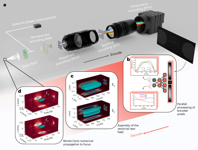
a, Optical setup task encodes the four-dimensional vector field onto a two-dimensional intensity measurement (not to scale). The collimated beam is split, with one part used to measure the spectral phase and the rest passing through a birefringent medium (BM), creating a relative spectral chirp between the polarizations. Next, a microlens array (MLA) encodes the wavefront. The resulting pattern is imaged by a 4f system with a diffraction grating (DG) placed near the Fourier plane, providing the spectral encoding, and a polarization filter array (PFA) is used on the sensor. b, Extraction and processing of the encoding pixels. At each point in space, the spectral and polarization information is recovered, with uncertainty estimates. c, Aggregation of the information from the encoder pixels into the vectorial near field. d, Propagation to focus.

The design begins with the Shack–Hartmann sensor²⁹. A common way to simultaneously capture the monochromatic intensity and phase of a laser pulse is by a microlens array, which locally samples the wavefront in many locations and encodes the average phase gradient over each sub-aperture into the resulting shifts of the focal spots. This averaging is crucial, as it both reduces aliasing from higher-frequency components and leads to a better signal-to-noise ratio compared with other phase-encoding methods, for example, the pinhole-based Hartmann sensor. To extend this to a hyperspectral setting, the plane of the focii is imaged using a 4f system, with a diffraction grating placed close to the Fourier plane. The resulting diffraction pattern at the sensor is composed of the fundamental order, as well as the ±1 orders, resulting in a kind of sparse tomography. Crucially, the ±1 orders obtain chromatic dispersion, thereby encoding the spectral information in streaks at the detector. Analogous to tomographic reconstruction, we can see these as projections of our hyperspectral intensity. One notes that it is necessary to have both ±1 orders, as with just one, there exists an ambiguity between the spectral intensity and phase.

To capture the full information of the polarization state and, thus, the four Stokes parameters, one must acquire the magnitudes of the field in two orthogonal directions, namely, ∥E_x∥ and ∥E_y∥, and the relative phase delay between them, δ. Here a camera with a polarizing filter array is used, which gives the spatial intensity for filters arranged in directions ∈ (0°, 45°, 90°, 135°). The field magnitudes are found as the square root of the 0° and 90° components. The magnitude of polarization delay is found by

where I is the intensity, but crucially, its sign is still unknown³⁰. Resultingly, the fourth Stokes parameter is only known to a plus–minus ambiguity, corresponding to an insensitivity to the handedness of the polarization state.

Here this is resolved by the prior knowledge of the signal’s sparsity, and the use of a precharacterized birefringent medium placed before the microlens. This element adds a further delay between the polarizations, δ_B, so that the final delay at the sensor is δ_M = δ + δ_B. From the assumption of the initial field’s smoothness, it follows that its initial spectral variation of the polarization delay, that is, \(\left\Vert \frac{\partial \delta }{\partial \lambda }\right\Vert\), is small. One chooses a birefringent medium that causes a large temporal chirp between the polarizations, such that \(\left\Vert \frac{\partial {\delta }_{{\rm{B}}}}{\partial \lambda }\right\Vert \gg \left\Vert \frac{\partial \delta }{\partial \lambda }\right\Vert\). When a measurement is taken, two ambiguous solutions are found, ±δ_M. Here one selects the solution whose spectral gradient is in the same direction as that of the birefringent medium. Subsequently, subtracting the precalibrated δ_B yields the initial field’s polarization delay δ. An example of a suitable birefringent medium is a multiorder half-wave plate, but with prior knowledge of the pulse’s expected polarization state, one can choose a medium to maximize the intensity in all four polarization channels to improve the signal-to-noise ratio.

Software decoder

Due to the unique encoding achieved by the optical setup, the system is theoretically bijective. However, real-world measurements invariably contain noise, which complicates the reconstruction process. Although convex optimization techniques could be used, they are typically slower and less adept at handling noise and uncertainty estimation. Thus, to achieve a real-time diagnostic capability that matches the repetition rate of ultraintense laser systems, neural networks are used. This approach not only provides rapid reconstruction (taking <0.1 s for the near field) but also excels at denoising the data and estimating uncertainties in the reconstruction. For the following discussion, the spatiotemporal indices (x, y, λ/t) are suppressed for brevity as they apply to every variable—conversely, where the indices are shown, they are the sole indices.

The reconstruction process begins by the extraction and subsequent analysis of the encoder pixels. These are formed of the microlens focii in the fundamental order (found using a peak finder), and the streaks in the ±1 orders, extracted using the precalibrated dispersion curve of the grating. The encoding pixels are then analysed in parallel by a fully connected deep neural network, which makes a prediction for the intensity in each polarization axis, I = [I₀, I₄₅, I₉₀, I₁₃₅], and the derivatives of the wavefront, \({\boldsymbol{\nabla }}{{\bf{\upphi }}}_{{\boldsymbol{x}}}=\left[\frac{\partial {\phi }_{x}}{\partial x},\frac{\partial {\phi }_{x}}{\partial y}\right]\), at each wavelength λ. By assuming a distribution of the uncertainty, one can train a network to estimate both values and their uncertainty, by minimizing the negative log-likelihood^31,32. Here the standard Gaussian is used for the wavefront derivatives, and the folded Gaussian³³ is used on the intensity to ensure that values below 0 are forbidden.

The vectorial near field is then formed by the synthesis of the encoding pixels. The phase derivatives for each wavelength are stitched together utilizing the zonal approach³⁴, yielding \({{\phi }^{{\prime} }}_{x}\). To obtain the spatiotemporal phase, the spectral phase must also be added: \({\phi }_{x}={{\phi }^{{\prime} }}_{x}+\tilde{\phi }(\lambda )\). The polarization delay δ is extracted from the intensity predictions, as described above, so that ϕ_y is then found as ϕ_y = ϕ_x – δ, without the need of a separate spectral phase measurement in the other polarization direction. The result of this analysis is the complete near field with uncertainty estimates.

It is the field at focus which is of the most physical importance. Thus, the measured near field, along with its uncertainty estimates, is numerically propagated to the focus. To propagate the uncertainty estimates, Monte Carlo sampling is used. For a number of iterations, the near field is sampled from its distribution and propagated to the far field, which is stored. Finally, the uncertainty of the field at focus is approximated as a Gaussian, by the calculation of the mean and standard deviation of the samples for each point in the spatiotemporal volume. The same process is applied to the desired derivatives of the field at focus, such as calculating the peak intensity. The following results use a Fresnel propagator since the pulses under scrutiny are focused with a long focal length. However, the spatiotemporal foci under strong focusing and the resulting longitudinal fields can also be reproduced using a Rayleigh–Sommerfeld propagator.

Measurements

Single-shot measurement of ultraintense laser pulses

The RAVEN technique was used to perform the single-shot measurements of the spatiotemporal vector field of petawatt-class laser pulses. Measurements were performed at the ATLAS-3000 facility, which, during our beamtime, generated pulses with up to 35-J energy and a pulse duration of 29.6 fs. The RAVEN characterization results are displayed in Fig. 2. Although all the polarization information is measured, only the field along the ATLAS’ main polarization axis is shown.

Fig. 2: Single-shot measurement of the spatiotemporal field of a petawatt-class laser pulse.

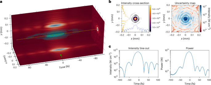
a, Electric field of an ATLAS-3000 pulse at focus. The visualization shows the isosurface of the field, where the carrier frequency has been reduced by factor of 2 for clarity. b, Temporal slice of the intensity at the centre of the beam (marked by the green arrow in a), along with its uncertainty estimate. Also included in the intensity slice are spatial line-outs through the centre of the cross-section, shown in the log scale. c, Intensity line-out through the centre of the beam, shown by the yellow line in a, and the power found by integrating the intensity over space. All the displayed error bars represent the predicted ±2σ confidence interval.

The resulting spatiospectral field at focus is shown in Fig. 2a, whereas a cut at t = 0 is shown in Fig. 2b. Note that the relative uncertainty at the peak intensity is two orders of magnitude lower than the signal level. Figure 2c shows the temporal intensity of the pulse, both at the focus position, (x = 0, y = 0), and integrated over space. The pulse duration of the former was found to be 29.8 ± 0.2 fs, in accordance with the previously quoted value. We calculated the spatiotemporal Strehl ratio of the laser (Methods)³⁵, which is a reduction in the peak intensity due to the wavefront. The absolute ratio was 0.81 and the STC-isolated ratio (taken by removing the spectrally averaged wavefront from the pulse) was 0.93. These values are similar to those quoted at other petawatt facilities³⁶.

After showing that RAVEN is able to resolve individual laser pulses, an experiment was performed to monitor, in real time, the STC content of the laser. Here the ATLAS-3000 system was operating at a 1-Hz repetition rate, whereas the pump energy was changed approximately every 20 min by changing the pump laser configuration. For each laser shot, RAVEN was used to acquire the pulse’s structure. We then calculate both STC content and STC-isolated spatiotemporal Strehl ratio, allowing the long-term dynamics of these changes to be studied. For these measurements, a reference was not taken, which means that the Strehl ratio includes the STCs induced by the optical system used to transport the pulse to RAVEN and is, thus, reduced compared with the true value. However, the dynamics can still be studied.

Figure 3 displays the evolution of the spatiotemporal Strehl ratio, along with the two STCs with the highest Pearson’s correlation coefficient with this ratio, namely, the pulse-front tilt in the horizontal direction (PFT_x) and the pulse-front curvature (PFC). It is apparent that the hyperspectral Strehl ratio generally improves with the pump energy; intuitively, this is due to the fact that the compressor is aligned at one pump energy for which the pulse-front tilt is minimized with an inverted field autocorrelator³⁷. Of all the STCs, it was found that PFT_x was the most strongly correlated to the peak intensity (Pearson's correlation coefficient ρ = 0.92).

Fig. 3: Evolution of the spatiotemporal Strehl ratio and STCs, with changes in the laser pump energy.

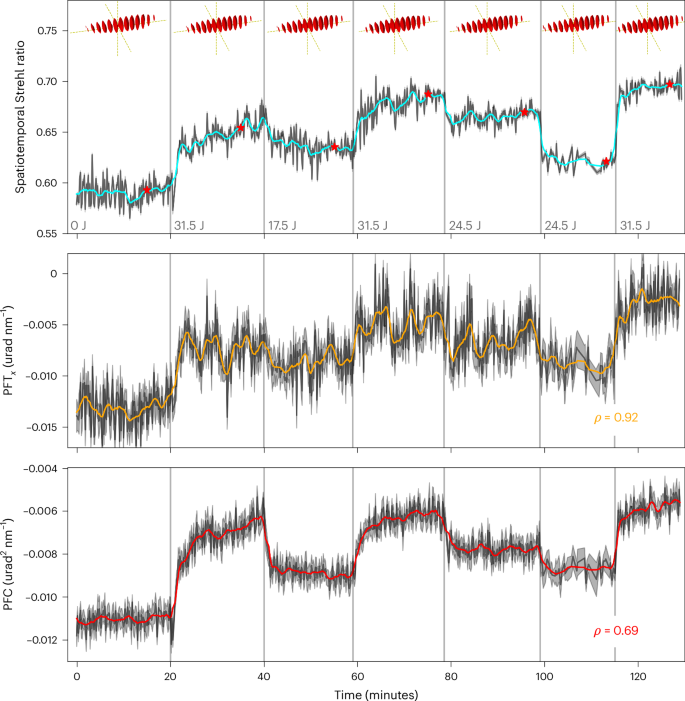
At each vertical grey line, the pump energy was changed, as denoted at the bottom of the spatiotemporal Strehl ratio subplot. Each red star denotes the temporal location in which the field is shown in the three-dimensional plot above. This measurement was not referenced, and thus, the spatiotemporal Strehl ratio includes contributions from STCs of the optical setup used to transport the pulse to the RAVEN setup.

PFC was also highly correlated, which displayed the property of stabilizing over relatively long time periods. This can be seen especially in the case when all the pump lasers were turned on, after they had all been off (T = 20 min). An explanatory candidate for this effect is the inhomogeneous heating of the gain medium as the pump energy was adjusted, and the subsequent change in thermal lensing³⁸. This lensing is in itself chromatic and will, thus, result in different pulse-front curvatures. To our knowledge, these subtle dynamics have not been previously observed, even though they have a non-negligible influence on the focused intensity, characterized by the spatiotemporal Strehl ratio.

Vector field characterization of optical vortices

To demonstrate the full capabilities of the RAVEN technique, an experiment was conducted to measure a laser pulse that requires a vectorial treatment. The optical vortex is a type of vector field that has the intriguing property of possessing orbital angular momentum, manifested by a spiral wavefront, which leads to the formation of the characteristic ‘doughnut’ focus on propagation. These attributes make it of high interest in many experiments in the high-intensity regime^39,40,41. Existing methods to characterize such fields have typically been developed for high-repetition-rate systems, requiring a scan with many laser shots^42,43.

Here a quarter-wave plate was used to circularly polarize the incoming laser pulse, before it passed through a vortex retarder, imparting the pulse with orbital angular momentum (m = 2). Considering the pulse in terms of its polarization components E_x and E_y, each possessing a spiral wavefront, with a \(\pm \frac{\uppi }{2}\) phase shift between them, with the sign depending on the handedness of the circular polarization. RAVEN utilizes a spectrally dependent birefringent medium (in this case, a simple half-wave plate), and the prior assumption of spectral smoothness to determine the handedness. Due to beamtime restraints, this experiment was performed on an ultrafast oscillator, but there is no reason why this would not work at an ultraintense facility. The results shown in Fig. 4 demonstrate the spectral dependence of the resultant vector field, as expected, due to the chromatic properties of the quarter-wave plate and vortex retarder used to generate it.

Fig. 4: Single-shot measurement of the spatiotemporal vector field of an optical vortex.

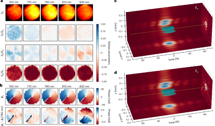
a, Spatiospectral Stokes parameters of the vectorial near field. b, Spiral wavefront of the optical vortex. The relative change from the design wavelength of the vortex retarder (780 nm) is also shown, displaying the chromatic properties of this object. c,d, Field at focus, for both E_x and E_y. The carrier frequency has been reduced by a factor of 2 for clarity, and the spatial units have been scaled to the ATLAS-3000 system (27-cm diameter in the near field).

In the case of a perfect left-handed circularly polarized beam⁴⁴, the final three normalized Stokes’ parameters have the values

Clear deviations from these values are seen as one moves away from the central wavelength of the laser because the quarter-wave plate is designed to create circularly polarized light at the design wavelength. Away from this, the polarization state will instead be elliptical. Similarly, one sees that deviations from the design wavelength of the vortex retarder leads to vortices being formed with non-integer orbital angular momentum.

In this work, we introduced RAVEN, a technique capable of the single-shot measurements of the spatiotemporal vector field of ultraintense laser pulses. In a paradigm shift from standard laser characterization devices, the development of RAVEN began with systematic considerations of the quantity of interest, the far field, which informed every subsequent design choice. The result is a method of superior capability and trustworthiness, providing a number of crucial benefits over previous work. Where most existing methods would require hundreds of shots, RAVEN achieves a complete spatiotemporal characterization of a laser pulse in just one, including full polarization information. This results in considerable time savings. Owing to its fast construction time, the method allows for online measurement and optimization at ultraintense laser facilities with repetition rates of ~1 Hz. This was demonstrated in its application to the ATLAS-3000 system, in a single-shot spatiotemporal vector field characterization of a petawatt-power laser pulse. Importantly, RAVEN facilitates the detection of phenomena that were previously inaccessible. This includes the shot-to-shot fluctuations of the spatiotemporal wavefront of the laser pulse. However, with the complete treatment of the polarization state of the pulse, vectorial ultraintense laser pulses can now be studied in real time.

We believe that the generality and numerous benefits of this technique will serve as a catalyst for advancing ultrafast physics, particularly in the realm of ultraintense lasers. RAVEN’s ability to provide comprehensive pulse characterization in real time enables the online optimization of laser parameters, enhancing the efficiency and effectiveness of experiments. This real-time capability paves the way for advanced optimization techniques, such as Bayesian optimization of laser-plasma acceleration⁴⁵, potentially leading to breakthroughs in particle acceleration and other applications. By offering crucial data on actual system performance, including shot-to-shot fluctuations and polarization information, RAVEN bridges the gap between simulation and experimental reality, improving the predictive power of computational models in ultraintense laser physics.

Importantly, RAVEN’s capability to fully characterize vector beams opens up new possibilities for using structured light in ultraintense laser experiments. This could lead to novel applications in areas such as particle acceleration, high-harmonic generation and laser-driven fusion, where precise control over the spatial, temporal and polarization properties of the laser pulse is crucial. The single-shot, full-vector-field characterization allows for the observation of subtle effects and transient phenomena that were previously undetectable, potentially driving improvements in laser design and control.

In conclusion, RAVEN not only provides a powerful new tool for laser diagnostics but also has the potential to accelerate progress across a wide range of ultraintense laser applications. By enabling the use and characterization of structured light beams in these extreme regimes, RAVEN opens up new avenues for controlling and manipulating light–matter interactions at the highest intensities, promising to push the boundaries of laser science and technology.

Validity of Fresnel regime

The design of the RAVEN technique is based on the principle that the level of confinement of the power spectrum of the pulse means that the resolutions required to capture it are much lower than those used in conventional devices. The necessary resolutions are calculated assuming propagation in the Fresnel regime, which means that focusing is described by a Fourier transform and Nyquist sampling theorem can be used to find the resolution. Some may argue that the strong focusing of an ultraintense laser pulse should instead be described by Rayleigh–Sommerfeld propagation, or even by non-classical physical laws. However, our argument and measurement process remain unaffected by this distinction. Our measurements occur in the near field, where the paraxial approximation is valid. As long as we can make assumptions about the ultraintense laser pulse’s power spectrum, that is, which volume the pulse would occupy when focused in the Fresnel regime, we can infer the properties of the underlying coherence structure in the near field. We can, therefore, also make statements about pulses under strong focusing, as long as we have a valid propagator that links our near-field results to the focus.

ATLAS-3000 measurements

The ATLAS system at the Centre for Advanced Laser Applications, Garching, is a state-of-the-art multipetawatt laser system designed for high-intensity laser–matter interaction experiments. Although capable of amplifying pulses up to 90 J, the maximum energy in this study was deliberately limited to 35 J to ensure machine safety, due to the presence of a hotspot in the near-field profile. For the results presented in this manuscript, the laser system was operated at pulse energies ranging from 15 J to 35 J, with energy variation achieved by adjusting the pump energy. The beam diameter in the near field is approximately 28 cm. The quoted intensity and power measurements in Fig. 2 also incorporate the combined efficiency of the compressor and beam transport system of ~70%.

During all the measurements, the beam was attenuated before compression using a reflective attenuator. It was then directed onto the RAVEN diagnostic setup, installed in one of the target chambers normally used for laser-plasma acceleration experiments. Within this setup, the beam was focused using a spherical mirror with a 10-m focal length and subsequently recollimated after the focus using an achromatic lens system. A beamsplitter within the imaging setup allowed for the simultaneous operation of the FALCON diagnostic. Furthermore, for the measurement shown in Fig. 2, a reference measurement was taken by placing a pinhole at the focus of the spherical mirror. Subtracting this reference wavefront from the real measurement allows for the removal of aberrations that are due to the optical system that carries the beam to the RAVEN setup.

The spectral phase was characterized using self-referenced spectral interferometry⁴⁶ with a commercial WIZZLER device immediately after the compressor. To optimize the experimental workflow, spectral phase measurements were conducted immediately following the RAVEN measurements, rather than simultaneously. This approach was justified by the observed high shot-to-shot stability of the spectral phase. Consequently, the intensity measurements presented in Fig. 2 incorporate the spectral phase data from a shot taken in close temporal proximity. It is worth noting that this sequential measurement strategy was adopted to efficiently utilize the available beamtime and does not reflect any inherent limitation of the RAVEN technique. Future implementations could readily incorporate simultaneous spectral phase measurements if deemed necessary for specific experimental objectives.

The pulse is propagated to the far field using a Fourier-based propagator (Supplementary Section 4.6). Naturally, the near field can be zero padded to increase the resolution of the pulse at focus, resulting in a grid with cells of size (Δx_focus, Δy_focus, Δt_focus). The intensity is then calculated with respect to these cells. The spatiotemporal Strehl ratio describes the reduction in the peak intensity of the pulse, compared with a pulse of the same spectrum, but having a flat phase. Here we consider two definitions³⁶. First, the absolute ratio is found by numerically propagating the pulse to focus and then calculating its peak intensity, and dividing this by the peak intensity of a pulse of equal spectra, but with a flat wavefront. To calculate the STC-isolated ratio, one considers the case of perfect separate spatial and temporal corrections to the pulse. This is found by making the spectrally averaged wavefront flat (for example, by a deformable mirror), as well as the spectral phase equal to 0 (by a DAZZLER). The pulse is then propagated to focus, and its peak intensity is divided by that of an identical pulse with a flat wavefront.

Long-term dynamics

In this experiment, the energy of the pump lasers was adjusted as the effect on the pulse structure was measured with RAVEN. Once the near field is acquired, two quantities are extracted. First, the STC content of the pulse, found by the modal decomposition of the spatiospectral wavefront into the Zernike–Taylor basis⁴⁷ (Supplementary Section 4.7). The second quantity was the spatiotemporal Strehl ratio of the pulse. For both quantities, the uncertainty estimates are found via Monte Carlo sampling. At T = 100, one sees a large change in the PFT, PFC and spatiotemporal Strehl ratio, despite it appearing that the pump energy remained constant. The main amplification stage of ATLAS is composed of two amplifiers; at T = 100 min, a pump laser from the first amplifier was switched off and another was switched on in the second amplifier, thereby changing the thermal load of each crystal.

References

Authors and Affiliations

1. Department of Physics, Clarendon Laboratory, University of Oxford, Oxford, UK

   Sunny Howard, Robin H. W. Wang, Peter Norreys & Andreas Döpp

2. Fakultät für Physik, Ludwig-Maximilian-Universität München, Garching, Germany

   Sunny Howard, Jannik Esslinger, Nils Weiße, Jakob Schröder, Christoph Eberle, Stefan Karsch & Andreas Döpp

3. Max Planck Institut für Quantenoptik, Garching, Germany

   Stefan Karsch & Andreas Döpp

4. John Adams Institute for Accelerator Science, Oxford, UK

   Peter Norreys

Contributions

S.H., J.E., N.W., J.S., C.E., R.H.W.W. and A.D. contributed to the method development and device calibration. S.H., N.W., J.E. and A.D. performed the measurements. S.H. analysed the results. All authors discussed the results. S.H. and A.D. wrote the paper. P.N. and A.D. supervised the project.

Corresponding author

Correspondence to Andreas Döpp.

Competing interests

The authors declare no competing interests.

Peer review information

Nature Photonics thanks Cord Arnold and Cheonha Jeon for their contribution to the peer review of this work.

Open Access This article is licensed under a Creative Commons Attribution 4.0 International License, which permits use, sharing, adaptation, distribution and reproduction in any medium or format, as long as you give appropriate credit to the original author(s) and the source, provide a link to the Creative Commons licence, and indicate if changes were made. The images or other third party material in this article are included in the article’s Creative Commons licence, unless indicated otherwise in a credit line to the material. If material is not included in the article’s Creative Commons licence and your intended use is not permitted by statutory regulation or exceeds the permitted use, you will need to obtain permission directly from the copyright holder. To view a copy of this licence, visit http://creativecommons.org/licenses/by/4.0/.

Reprints and permissions

References

Danson, C. N. et al. Petawatt and exawatt class lasers worldwide. High Power Laser Sci. Eng. 7, e54 (2019).
Zeng, X. et al. Multi-petawatt laser facility fully based on optical parametric chirped-pulse amplification. Opt. Lett. 42, 2014–2017 (2017).
Sung, J. H. et al. 4.2 PW, 20 fs Ti:sapphire laser at 0.1 Hz. Opt. Lett. 42, 2058–2061 (2017).
Radier, C. et al. 10 PW peak power femtosecond laser pulses at ELI-NP. High Power Laser Sci. Eng. 10, e21 (2022).
Yoon, J. W. et al. Realization of laser intensity over 1023 W/cm2. Optica 8, 630–635 (2021).
Alonso, B., Döpp, A. & Jolly, S. W. Space–time characterization of ultrashort laser pulses: a perspective. APL Photon. 9, 070901 (2024).
Akturk, S., Gu, X., Bowlan, P. & Trebino, R. Spatiotemporal couplings in ultrashort laser pulses. J. Opt. 12, 093001 (2010).
Dorrer, C. Spatiotemporal metrology of broadband optical pulses. IEEE J. Sel. Topics Quantum Electron. 25, 3100216 (2019).
Jolly, S. W., Gobert, O. & Quéré, F. Spatiotemporal characterization of ultrashort laser beams: a tutorial. J. Opt. 22, 103501 (2020).
Shen, Y. et al. Roadmap on spatiotemporal light fields. J. Opt. 25, 093001 (2023).
Zhan, Q. Spatiotemporal sculpturing of light: a tutorial. Adv. Opt. Photon. 16, 163–228 (2024).
Jolly, S. W. Focused fields of ultrashort radially polarized laser pulses having low-order spatiotemporal couplings. Phys. Rev. A 103, 033512 (2021).
Bourassin-Bouchet, C., Stephens, M., de Rossi, S., Delmotte, F. & Chavel, P. Duration of ultrashort pulses in the presence of spatiotemporal coupling. Opt. Express 19, 17357–17371 (2011).
Li, Z., Tsubakimoto, K., Yoshida, H., Nakata, Y. & Miyanaga, N. Degradation of femtosecond petawatt laser beams: spatiotemporal/spectral coupling induced by wavefront errors of compression gratings. Appl. Phys. Express 10, 102702 (2017).
Kong, F., Larocque, H., Karimi, E., Corkum, P. B. & Zhang, C. Generating few-cycle radially polarized pulses. Optica 6, 160–164 (2019).
Zaïm, N. et al. Interaction of ultraintense radially polarized laser pulses with plasma mirrors. Phys. Rev. X 10, 041064 (2020).
Forbes, A., de Oliveira, M. & Dennis, M. R. Structured light. Nat. Photon. 15, 253–262 (2021).
Sainte-Marie, A., Gobert, O. & Quéré, F. Controlling the velocity of ultrashort light pulses in vacuum through spatio-temporal couplings. Optica 4, 1298–1304 (2017).
Froula, D. H. et al. Spatiotemporal control of laser intensity. Nat. Photon. 12, 262–265 (2018).
Caizergues, C., Smartsev, S., Malka, V. & Thaury, C. Phase-locked laser-wakefield electron acceleration. Nat. Photon. 14, 475–479 (2020).
Genty, G. et al. Machine learning and applications in ultrafast photonics. Nat. Photon. 15, 91–101 (2021).
Döpp, A. et al. Data-driven science and machine learning methods in laser–plasma physics. High Power Laser Sci. Eng. 11, e55 (2023).
Hatfield, P. W. et al. The data-driven future of high-energy-density physics. Nature 593, 351–361 (2021).
Walmsley, I. A. & Dorrer, C. Characterization of ultrashort electromagnetic pulses. Adv. Opt. Photon. 1, 308–437 (2009).
Kim, Y. G. et al. Single-shot spatiotemporal characterization of a multi-PW laser using a multispectral wavefront sensing method. Opt. Express 29, 19506–19514 (2021).
Howard, S., Esslinger, J., Wang, R. H., Norreys, P. & Döpp, A. Hyperspectral compressive wavefront sensing. High Power Laser Sci. Eng. 11, e32 (2023).
Tang, H. et al. Single-shot compressed optical field topography. Light Sci. Appl. 11, 244 (2022).
Goodman, J. W. Introduction to Fourier Optics (Roberts and Company Publishers, 2005).
Platt, B. C. & Shack, R. History and principles of Shack-Hartmann wavefront sensing. J. Refract. Surg. 17, S573–S577 (2001).
Lane, C., Rode, D. & Rösgen, T. Calibration of a polarization image sensor and investigation of influencing factors. Appl. Opt. 61, C37–C45 (2022).
Nix, D. A. & Weigend, A. S. Estimating the mean and variance of the target probability distribution. In Proc. 1994 IEEE International Conference on Neural Networks (ICNN’94) 55–60 (IEEE, 1994).
Skafte, N., Jørgensen, M. & Hauberg, S. Reliable training and estimation of variance networks. Adv. Neural Inf. Process. Syst. 32, 1–11 (2019).
Leone, F. C., Nelson, L. S. & Nottingham, R. B. The folded normal distribution. Technometrics 3, 543–550 (1961).
Southwell, W. H. Wave-front estimation from wave-front slope measurements. J. Opt. Soc. Am. 70, 998–1006 (1980).
Pariente, G., Gallet, V., Borot, A., Gobert, O. & Quéré, F. Space–time characterization of ultra-intense femtosecond laser beams. Nat. Photon. 10, 547–553 (2016).
Jeandet, A. et al. Spatiotemporal structure of a petawatt femtosecond laser beam. J. Phys. Photon. 1, 035001 (2019).
Pretzler, G., Kasper, A. & Witte, K. J. Angular chirp and tilted light pulses in CPA lasers. Appl. Phys. B 70, 1–9 (2000).
Cho, S., Jeong, J., Hwang, S. & Yu, T. J. Thermal lens effect model of Ti:sapphire for use in high-power laser amplifiers. Appl. Phys. Express 11, 092701 (2018).
Wang, W. P. et al. Hollow plasma acceleration driven by a relativistic reflected hollow laser. Phys. Rev. Lett. 125, 034801 (2020).
Aboushelbaya, R. et al. Orbital angular momentum coupling in elastic photon–photon scattering. Phys. Rev. Lett. 123, 113604 (2019).
Vieira, J. et al. Amplification and generation of ultra-intense twisted laser pulses via stimulated Raman scattering. Nat. Commun. 7, 10371 (2016).
Alonso, B. et al. Complete spatiotemporal and polarization characterization of ultrafast vector beams. Commun. Phys. 3, 151 (2020).
Zdagkas, A., Nalla, V., Papasimakis, N. & Zheludev, N. I. Spatiotemporal characterization of ultrashort vector pulses. APL Photon. 6, 116103 (2021).
Rosales-Guzmán, C., Ndagano, B. & Forbes, A. A review of complex vector light fields and their applications. J. Opt. 20, 123001 (2018).
Irshad, F. et al. Pareto optimization and tuning of a laser wakefield accelerator. Phys. Rev. Lett. 133, 085001 (2024).
Oksenhendler, T. et al. Self-referenced spectral interferometry. Appl. Phys. B 99, 7–12 (2010).
Weisse, N. et al. Measuring spatiotemporal couplings using modal spatio-spectral wavefront retrieval. Opt. Express 31, 19733–19745 (2023).
Acknowledgements
We thank the Federal Republic of Germany and the Free State of Bavaria for funding the CALA infrastructure (15171 E 0002) and its operation. This work was supported by the Independent Junior Research Group ‘Characterization and control of high-intensity laser pulses for particle acceleration’, DFG Project No. 453619281. N.W. is funded by the EU Horizon 2020 IMPULSE project (Grant No. 87116). C.E. is funded by BMBF through the MACLIP project. We would also like to acknowledge UKRI-STFC grant ST/V001655/1. We acknowledge useful discussions with Professor Peter Norreys’ group. We thank Professor Stefan Karsch’s group for providing access and operation of the ATLAS-3000 system.
Ethics declarations