.png)

Graph Neural Networks (GNN) are a powerful and an increasingly popular technology, be it for Protein Folding and Discovery, Social Network Recommendations, Relational Deep Learning, or one of countless other practical applications. Their ability to process graph-shaped data makes them suitable for task types that other machine learning algorithms cannot handle, such as learning from complicated interactions and dependencies.
When trying to apply them in production, one can quickly hit a major scaling challenge. Real world datasets and databases can contain up to billions of nodes that cannot physically be loaded on a GPU. To make these models work in practice, we need to sample the graph to a manageable size - and this is where graph sampling comes in! To make accurate predictions for a node, we do not need to process the entire database! The most relevant information to a node is usually found in its immediate neighborhood and we can reduce the size of the graph by only processing the closest and most recent neighbors by using sampling algorithms such as GraphSAGE.
In this blog we will introduce the GraphSAGE sampling algorithm, typically used in Relational Deep Learning and how to set up a good sampling configuration. Secondly, we will take a look at the Kumo-developed adaptive metapath-aware graph sampling algorithm that improves GraphSAGE and addresses its shortcomings, adding up to 50% relative improvement on popular benchmarks!
GraphSAGE in Relational Deep Learning
GraphSAGE is a pioneering algorithm in the field of graph neural networks that enables efficient learning on large-scale graphs. It works by sampling a fixed number of neighbors for each node. The sampling process happens in steps, where at each step we sample neighbors from the nodes obtained in the previous step. By limiting the number of neighbors at each step, we create a computational graph that is both memory-efficient and scalable to large datasets.
Let us look at an illustrative example of a retailer database schema:
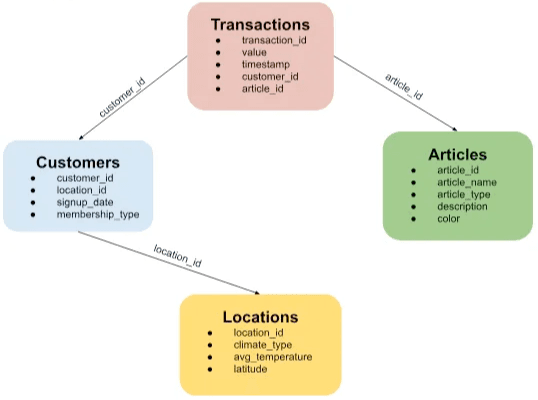
A schema of an example retailer dataset of customers, transactions, articles, and locations. In such datasets, past purchasing patterns are usually a better predictor of future purchases than location.
Suppose that we are trying to predict future purchases of an individual customer with the following neighbor sampling configuration in Kumo:
yaml
num_neighbors: - hop1: customers.customer_id->transactions.customer_id: 10 customers.customer_id->locations.location_id: 1 hop2: transactions.article_id->articles.article_id: 1 locations.location_id->customers.customer_id: 2The algorithm follows three key steps:
- We start from the customer that the prediction is made for.
- At every hop, we add the specified number of neighbors into the graph:
- In hop 1, we will add the customer’s location and their latest 10 transactions.
- In hop 2, we will sample the corresponding article for each transaction and 2 customer profiles from the same location.
- Collect all the sampled nodes into a new graph and use them as the input to the GNN model.
The resulting output after the above process should look like this 24-node graph:
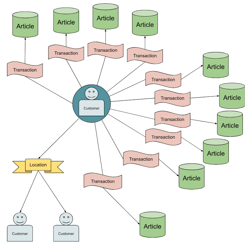
Expected output sample of GraphSAGE algorithm with the above simple config.
However, complex tasks such as purchase prediction and article recommendation benefit from a larger context. To obtain richer predictions, we want the model to benefit from collaborative filtering: including articles purchased by other customers with a similar purchase history and location. Moreover, we expect that purchase history is a more indicative signal of customer similarity than location and want to sample our graph accordingly: sample more nodes based on the customer purchase history than based on location.
To achieve the above, we may choose to use a more sophisticated setup that explores graph over six hops:
yaml
num_neighbors: - hop1: customers.customer_id->transactions.customer_id: 10 customers.customer_id->locations.location_id: 1 hop2: transactions.article_id->articles.article_id: 1 locations.location_id->customers.customer_id: 2 hop3: articles.article_id->transactions.article_id: 10 customers.customer_id->transactions.customer_id: 10 hop4: transactions.article_id->articles.article_id: 1 transactions.customer_id->customers.customer_id: 1 hop5: articles.article_id->transactions.article_id: 10 customers.customer_id->locations.location_id: 1 customers.customer_id->transactions.customer_id: 10 hop6: transactions.customer_id->customers.customer_id: 1 locations.location_id->customers.customer_id: 2 transactions.article_id->articles.article_id: 1The configuration above might seem daunting, but it is constructed by following three very simple rules:
- All foreign key to primary key connections only sample 1 neighbor since there is only one to sample.
- All locations → customers connections are set to 2 because we expect that they provide less information compared to other connection types.
- All other primary key to foreign key connections are set to 10.
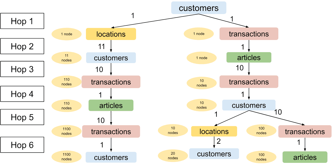
In the below illustration, we roll-out the 6 hops of sampling from the above config to demonstrate how the resulting sampled graph will look like. Numbers on arrows are the numbers from the config and indicate the number of sampled neighbors at each hop.
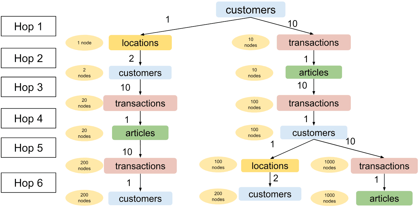
The expected output of GraphSAGE using a more sophisticated sampling setup. Numbers in the yellow ovals represent the expected number of sampled nodes of each type.
As evident from the numbers in the illustration, the number of sampled nodes increases exponentially and we end up with a graph with almost 3000 nodes. Recklessly setting the number of neighbors to large values can slow down the training or even cause memory issues so it is important to be mindful when using a larger number of hops.
In the above scenario, the numbers have been carefully chosen to ensure that majority of sampled nodes come from the exploration of purchasing patterns of customers with a similar history. Moreover, the size of the graph is still small enough that the model will train within a reasonable time and without hiccups.
Drawbacks of GraphSAGE Sampling
However, while GraphSAGE is efficient and widely used, its uniform sampling strategy may not be optimal for heterogeneous graphs derived from relational databases. The requirement to sample a static number of neighbors per hop is unnecessarily rigid and does not adapt well to different input examples.
In the H&M article purchase dataset, about 20% of customers have fewer than 5 articles in their purchase history, while 45% have 20 or more.
A fixed configuration unavoidably fails both of these groups:
If the customer has a very long history, it can be more helpful to learn from their past purchasing patterns instead of only last 10 transactions, even if that means sampling fewer neighbors in later hops.
If the customer has a very short history, we end up sampling much fewer nodes in the first hop, under-utilizing the available resources. Let us take a look at the sampling diagram for a customer with only one past transaction:
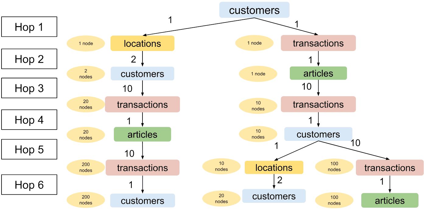
The expected output of GraphSAGE for a customer with only one past transaction. We end up sampling much fewer nodes, underutilizing the available resources.
We have sampled less than 15% of the graph size compared to the optimal case, with most of the sampled nodes coming from customers at the same location - the neighborhood that is less relevant to the overall prediction!
A naive attempt to fix this resource under-utilisation might be to oversample in the second hop whenever we under-sample nodes in the first hop. Or more generally, oversample in hop whenever we do not sample the expected number of nodes in hop .
In the above example, there is only edge type in the second hop where more than 1 neighbor can be sampled. That is the edge type locations.location_id->customers.customer_id. Sampling the additional 9 nodes there leads to the following sampled graph:
A naive and incorrect solution to the problem of rigid sampling for the customer with only one transaction: Oversampling at step 2 over-samples the subtree that we consider less informative.
This solution only makes the situation worse - it increases the size of the left and less relevant subtree!
Adaptive Metapath-aware Graph Sampling
An approach that avoids this pitfall needs to be aware of the metapath of the missing nodes. When trying to make up for missing samples, it should sample exactly the types of nodes that would otherwise be missing from the final graph sample.
- If the sampler does not manage to sample the planned number of neighbors in a hop, it tries to oversample other neighbors with the same metapath. For example, if we wanted to sample 10 last purchases of each article that a customer bought, but one item has only been purchased twice, we make up for this by oversampling past purchases of other items that this customer bought.
- If this is not possible, we oversample children of nodes with the same path. For example, if the customer only had one historical transaction (instead of 10), we will oversample neighbors of that transaction and its corresponding article.
Let’s return back to the example of a customer with a single transaction. We are using the same model plan as above:
yaml
num_neighbors: - hop1: customers.customer_id->transactions.customer_id: 10 # only one transaction sampled successfully customers.customer_id->locations.location_id: 1 hop2: transactions.article_id->articles.article_id: 1 locations.location_id->customers.customer_id: 2 hop3: articles.article_id->transactions.article_id: 10 customers.customer_id->transactions.customer_id: 10 hop4: transactions.article_id->articles.article_id: 1 transactions.customer_id->customers.customer_id: 1 hop5: articles.article_id->transactions.article_id: 10 customers.customer_id->locations.location_id: 1 customers.customer_id->transactions.customer_id: 10 hop6: transactions.customer_id->customers.customer_id: 1 locations.location_id->customers.customer_id: 2 transactions.article_id->articles.article_id: 1This is how the sampled subgraph is expected to look like when following the above logic:
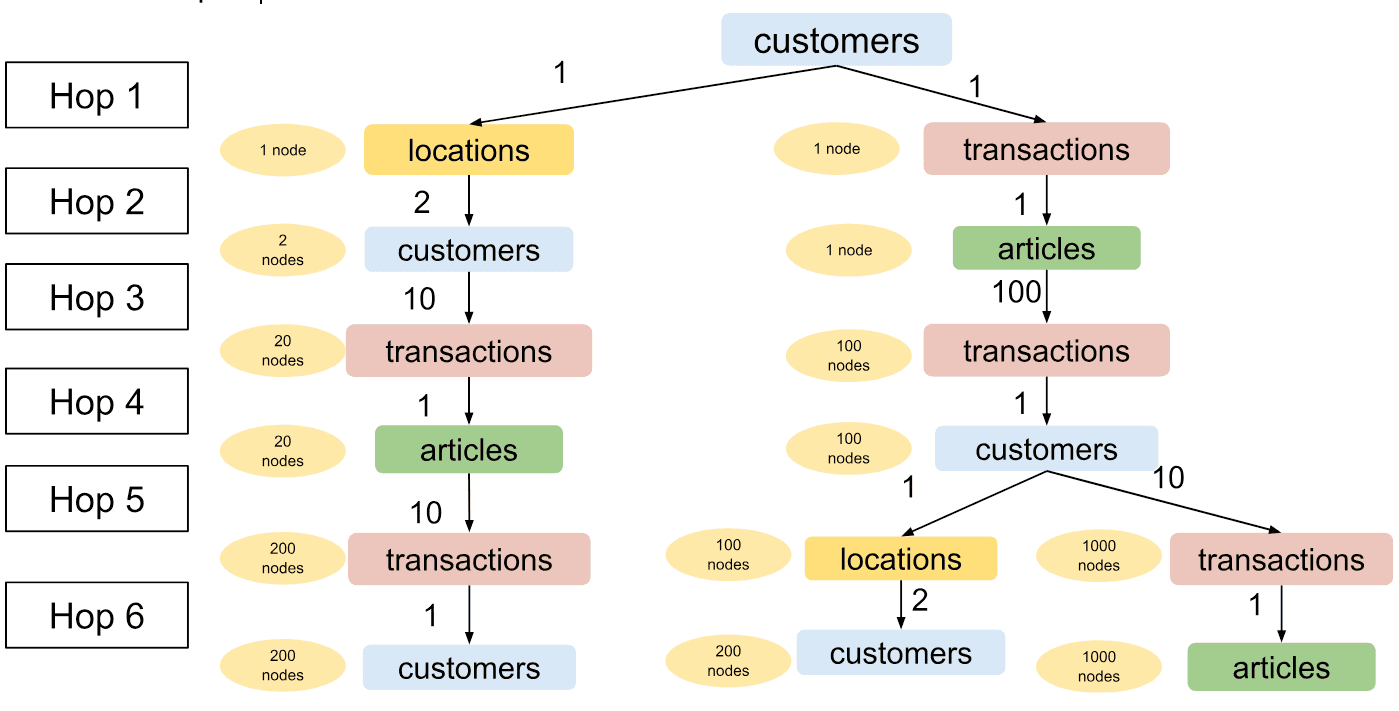
Sampled graph using Adaptive Metapath-Aware Sampling for a customer with single item purchase history.
To make up for the lack of transaction history, the sampler selected 100 past buyers of the only item that the customer bought, keeping the balance of the tree.
Let us take a look at another example with the same config as above. Suppose that a customer only had two past transactions items A and B. However, they were both added to the database recently and only had a short history of purchases; item A was purchased 5 times and item B 45 times. After hop 1, we will have only 2 sampled transactions instead of the specified 10. Even by sampling all past purchases of items A and B, we will only manage to sample 50 transactions in hop 3 — 5 history transactions of item A and 45 of item B. We will compensate for this in each of the two subtrees in the bottom right part of the image. We double the number of sampled transactions per past customer in hop 5 and double the number of customers from a location in hop 6.
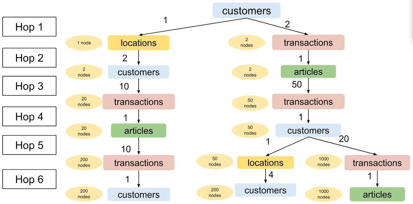
Sampled graph with Adaptive Metapath-Aware Sampling for a customer with 2 items in the purchase history where both of these items have only been purchased 50 times in total.
This resolves the issue for customers with short transaction histories.
Dealing with a Long Transaction History
Customers with very long transaction histories also benefit from adaptive sampling!
Knowing that the sampler is able meaningfully redistribute the sampling budget, we can safely set the number of neighbors in the first hop to a much larger number. In fact, all of our experiments in the analysis section were done with a very simple neighbor sampling setup:
yaml
num_neighbors: - hop1: customers.customer_id->transactions.customer_id: 1000 customers.customer_id->locations.location_id: 200 hop2: default: 1 hop3: default: 1 hop4: default: 1 hop5: default: 1 hop6: default: 1This configuration specifies to sample as much as possible in the first hop, and relies on the sampler to correctly redistribute the budget towards later hops.
Experimental Analysis
We test the algorithm on RelBench benchmark for relational deep learning. We specifically focus on the link prediction subset because it is known to benefit from additional hops. It is thus reasonable to expect that smarter sampling would improve the predictions.
We ran a single experiment for each setup with a fixed set of hyperparameters to obtain the following results:
| rel-amazon user-item-purchase | map@10 | 0.014 | 0.021 | 50% |
| rel-amazon user-item-rate | map@10 | 0.017 | 0.023 | 35.3% |
| rel-amazon user-item-review | map@10 | 0.013 | 0.019 | 46.1% |
| rel-avito user-ad-visit | map@12 | 0.031 | 0.036 | 16.1% |
| rel-hm user-item-purchase | map@12 | 0.030 | 0.032 | 6.7% |
| rel-stack post-post-related | map@100 | 0.120 | 0.110 | -8.3% |
| rel-stack post-post-comment | map@100 | 0.125 | 0.129 | 3.2% |
| rel-trial condition-sponsor-run | map@10 | 0.093 | 0.111 | 19.4% |
| rel-trial site-sponsor-run | map@10 | 0.244 | 0.251 | 2.9% |
The increase in performance is consistent across most tasks, on average adding 19% of relative improvement. On Amazon datasets it adds up to a 50% relative MAP@K boost!
To better understand where these improvements are coming from, let us take a closer look at H&M user-item-purchase task. H&M is a dataset with a very similar schema to the motivating example where the goal is to predict future purchases of a user based on their history. Let us compare performance gains for different users, grouped by the number of past transactions:
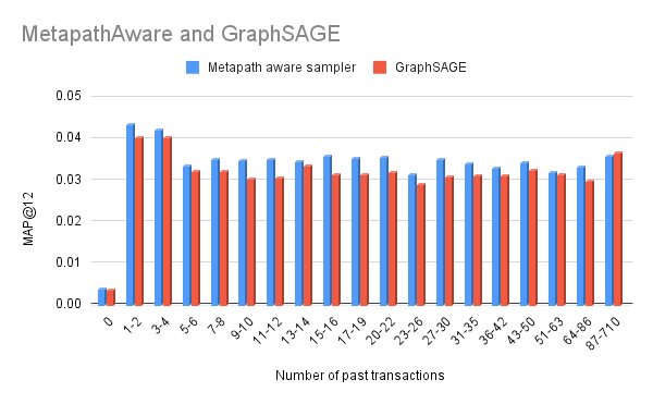
Comparison of GraphSAGE and Adaptive Metapath-aware Sampling performance by customer transaction history.
We can see that the performance improves across almost all groups. To our pleasant surprise, MAP@12 improves even in the user groups with approximately 10 past transactions where the fixed sampling configurations should work best. We can conclude that the metapath-aware adaptive sampling allows us not only to utilize the resources better, but to train more accurate models by making use of larger training samples.
When not to Use Adaptive Metapath-aware Graph Sampling
While the above results imply that adaptive sampling is usually beneficial to the prediction quality, it may not always be a good idea. The sampling setup needs at least two sequenced primary key to foreign key connections for adaptive sampling to take effect. In the H&M example, these connections were hop1: customers.customer_id->transactions.customer_id, followed by hop3: articles.article_id->transactions.article_id and hop5: customers.customer_id->transactions.customer_id. If a sampling setup uses fewer than 3 hops, there is likely no benefit from enabling adaptive sampling.
Another case where adaptive sampling is unlikely to help is when increasing the number of sampled neighbors in the config does not improve the model accuracy. This can happen in e.g. simple tasks where the most relevant information already appears in the user table, where sampling methods are not likely to affect the model quality.
Using adaptive sampling in the above scenarios might not necessarily reduce prediction quality, but it can significantly increase the computational costs for no good benefit.