.png)

While hardware-radio-using tools like the BTLEJACK excel at intercepting BLE connections, sniffing an already-established, frequency-hopping connection using a software-defined radio (SDR) presents some unique challenges, but also several opportunities.
Bluetooth Low Energy (BLE) is a wireless communication protocol designed for short-range applications where power consumption is a critical concern. This makes it the go-to technology for a vast ecosystem of Internet of Things (IoT) devices, including fitness trackers, smart home sensors, medical monitors, and asset tracking tags. From a security and reverse-engineering perspective, the ability to "listen in" on these communications is invaluable. It allows us to understand how devices talk to each other, discover proprietary protocols, and identify potential security vulnerabilities.
A Software Defined Radio (SDR) is a radio communication system where components that have been typically implemented in hardware (e.g., mixers, filters, modulators, demodulators) are instead implemented in software on an embedded system. In essence, an SDR acts as a highly versatile digital receiver. It tunes to a wide spectrum of frequencies and streams the raw radio data to a host computer, which can then process it to decode almost any wireless protocol, including BLE.
This blog post describes a methodology to sniff BLE communications using a relatively inexpensive SDR such as the HackRF One.
By reading this post, you will learn BLE/SDR basics and how we overcame the three main challenges we encountered:
- How to handle the difference in transmit power on both ends of the BLE connection
- How to follow the channel hopping despite the USB latency (since we cannot listen to all channels simultaneously)
- How to deduce the channel hopping scheme without seeing the frame that initiates the connection
We assume that the reader has some experience in C programming and basic math.
Before describing our approach, we will first cover BLE protocol and SDR basics. Please be aware that the information given in this post applies to the BLE 5.0 specifications.
The Bluetooth Low Energy protocol is organized in a stack of layers, similar to the OSI model for networking. In this post, we will focus on the Link-Layer (LL), which sits directly on top of the Physical Layer (PHY). The LL is responsible for managing the radio state, including advertising, scanning, and establishing and maintaining connections. It defines the packet structure, channel hopping, and timing that we will be exploring in detail.
The BLE link-layer protocol uses up to 40 radio channels, numbered from 0 to 39. Each channel is assigned its own frequency, and there are two types of channels:
- The Advertisement channels (numbered 37, 38, and 39) that serve as connection management (such as discovery and initiating connections)
- The Data channels (numbered 0 to 36) that carry the actual connection data after it's established
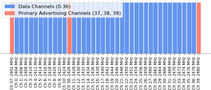 BLE channels and their frequencies
The devices participating in a BLE connection exchange packets on the various channels. The general structure of a packet is as follows:
| 1 byte | 4 bytes | variable size | 3 bytes |
The general structure of a PDU is as follows:
| 1 byte | 1 byte | variable size |
Advertisement PDUs are exchanged on the advertisement channels, and Data PDUs are exchanged on the data channels.
A BLE connection involves two roles:
- The Central: This is the device that initiates the connection (such as a smartphone or computer)
- The Peripheral: This is the service we connect to (such as a smart lightbulb or heart rate sensor)
The process of establishing the connection involves three phases:
Advertisement phase
The Peripheral device that wants to accept connections broadcasts ADV_IND packets at a regular interval (called the advertising interval) on the advertising channels in a round-robin fashion (i.e., on channel 37, then 38, then 39, then again 37, and so on).
Scanning phase
The Central device listens on the advertising channels to pick up ADV_IND packets.
Connection phase
When the Central device receives any ADV_IND packets from a device it wants to connect to, it replies with a CONNECT_IND packet to the Peripheral on the same advertising channel.
📝 Example: BLE connection establishment between two devices
Let's assume we've already found the Access Address (AA = 0xDEADBEEF) and the Connection Interval (connInterval = 37.5ms)...
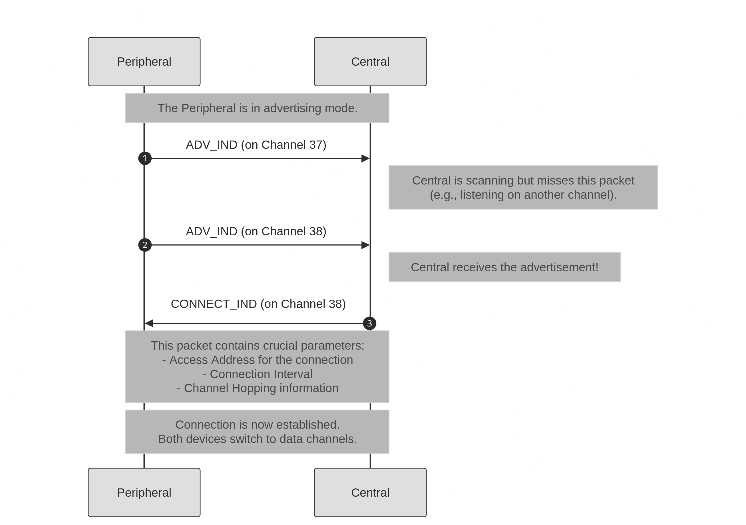 BLE connection sequence diagram
The CONNECT_IND packet contains some crucial information required for the subsequent data exchange. Here are the most important ones:
- The Access Address for the Data PDUs that will be exchanged on the connection
- The Connection Interval that specifies the interval at which the devices will exchange data
- The Channel Map, Hop Increment, and ChSel fields that specify the channel hopping scheme
There are two possible algorithms for the channel hopping scheme:
- Algorithm 1 is a simple algorithm that must be supported by all devices
- Algorithm 2 is a more complex algorithm that is used only when both devices participating in the connection support it
In this blog post, we will focus on Algorithm 2 since it is the more widely used in practice.
Once the Central and Peripheral devices have established a connection using the advertising channels, they switch to the data channels to exchange application data. This exchange is not a continuous stream but is structured into periodic bursts called connection events. During these events, the devices wake up, exchange one or more data packets, and then go back to sleep to conserve power.
In order to maintain a robust connection and avoid interference, BLE employs a channel hopping scheme, meaning the channel used changes for every connection event. Understanding how this data exchange is timed and how the channel hopping sequence is determined is fundamental to successfully sniffing an ongoing connection.
Connection timing properties
In this section, we will focus on the connection event timings, enabling us to understand the channel hopping in the next section.
Recall that the central and peripheral devices exchange packets during connection events, which consist of a sequence of exchanges. Each exchange is initiated by the central device by sending a packet, then the peripheral device replies, then the central device initiates the next exchange, and so on, until the connection event is terminated.
The time at which the first packet of a connection event is sent by the central device is called the anchor of this connection event. The time between two subsequent anchors is determined by the connection interval negotiated in the CONNECT_IND packet.
There may be a small amount of jitter affecting the timing of anchors. In that case, the timing of subsequent anchors shall be determined relative to the actual time of the last anchor.
📝 Example: Anchors and connection events
For instance, if:
- Anchor 1 happens at T
- Anchor 2 happens at T + connInterval + smallJitter
Then, Anchor 3 will be expected at T + connInterval + smallJitter + connInterval
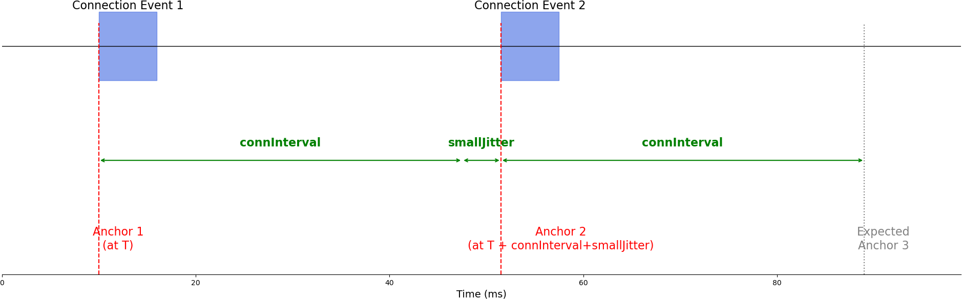 Chronogram of connection events
Channel hopping
At each connection event, the data channel changes. When using Algorithm 2 (as we assume), the picked channel depends on the following:
- The Access Address (AA) and the Channel Map negotiated at the start of the connection
- The connection event counter (incremented at each connection event)
The following schema describes the algorithm used to compute the channel number based on the AA and event counter.
🔍Closer look: Channel hopping algorithmLet's dive into the details of the channel hopping algorithm. These figures are taken from the Core 5.0 Bluetooth specifications.First, the channel identifier is computed as such: channelID = (AccessAddress & 0xFFFF) ^ (AccessAddress >> 16) Then, the connection event counter and the channel identifier are used to compute the channel index:
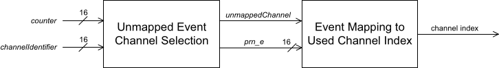 Computing the channel index
In that case, first, the remapping index is computed as such: remappingIndex = int((N*prn_e) / 65536) (where N is the number of used channels). The mapping process is shown here:
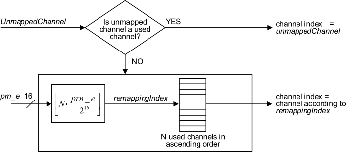 Remapping channel index
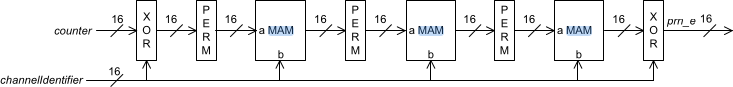 PRNG used in the channel hopping
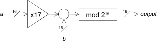 MAM operation
This section will cover SDR basics. Readers interested in more details are encouraged to read the excellent PySDR tutorials.
The SDR listens to radio waves and converts them into a format that can be handled by the host, in a process called IQ sampling that we will describe in more detail in the following section.
IQ sampling
The SDR device is commanded by the host (your PC) that instructs it to "tune" to an arbitrary frequency (called the center frequency).
Once the SDR is tuned to a frequency, it listens to the radio waves around that frequency and provides the host a stream of I and Q integer values, sampled at a specific interval (called the sampling rate).
The core mechanism of the IQ sampling is taking this "raw" radio wave and converting it into the stream of IQ values.
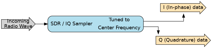 SDR producing IQ samples from radio waves
Joseph Fourier tells us that any signal can be represented as a sum of sine waves. To illustrate the concept, we will provide some examples of IQ sampling with radio sine waves to get the idea of what is done.
🔍Closer look: The Fourier TransformThe Fourier transform is a way to take something that changes over time (like a radio wave) and break it into the pure, sine waves that make it up. It tells you which frequencies are present and their respective strengths.Think of it like taking a musical chord and figuring out which individual notes are being played.
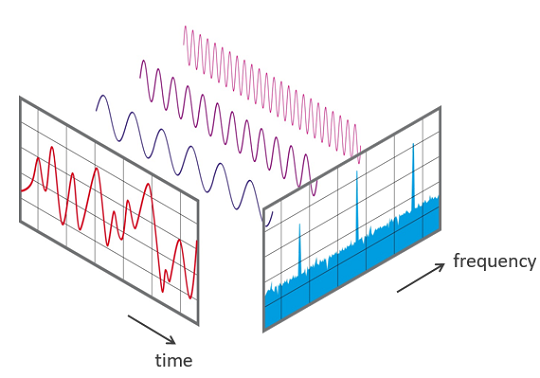 Fourier transform
A sine wave is characterized by its frequency (i.e., the frequency at which the signal "repeats itself"), its amplitude (i.e., the "strength" of the signal), and its phase (i.e., the time-shift relative to a pure sine wave).
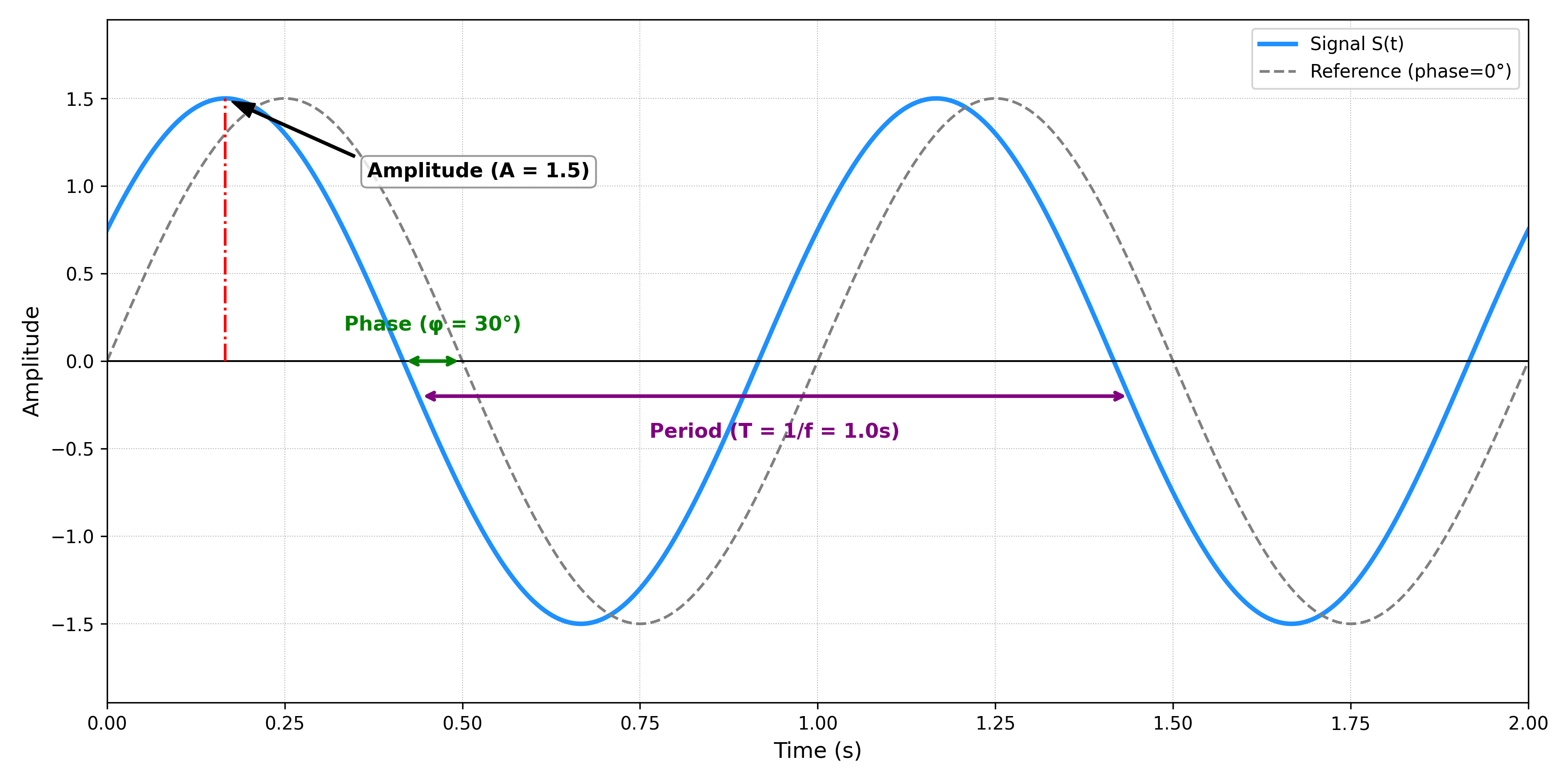 Sine wave with characteristics
In order to do the IQ sampling, the SDR generates two sine wave signals:
- The in-phase signal, which is a sine wave at the SDR's tuned frequency
- The quadrature-phase signal, which is the same sine wave as the in-phase signal, except it's time-shifted by a quarter of a period (i.e., it "lags" behind the in-phase signal by 90°)
For mathematical reasons, any sine waveS(t)can be expressed as:
I×inPhase(t)-Q×quadraturePhase(t)
.
But how areIandQrelated toS(t)? Let's make a few sample signals to find out.
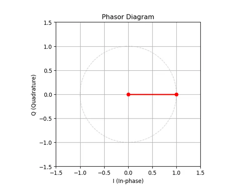
📝 Example: The case where S(t) is exactly equal to the in-phase signal. Relative to the in-phase signal, the phase of S(t) is 0.
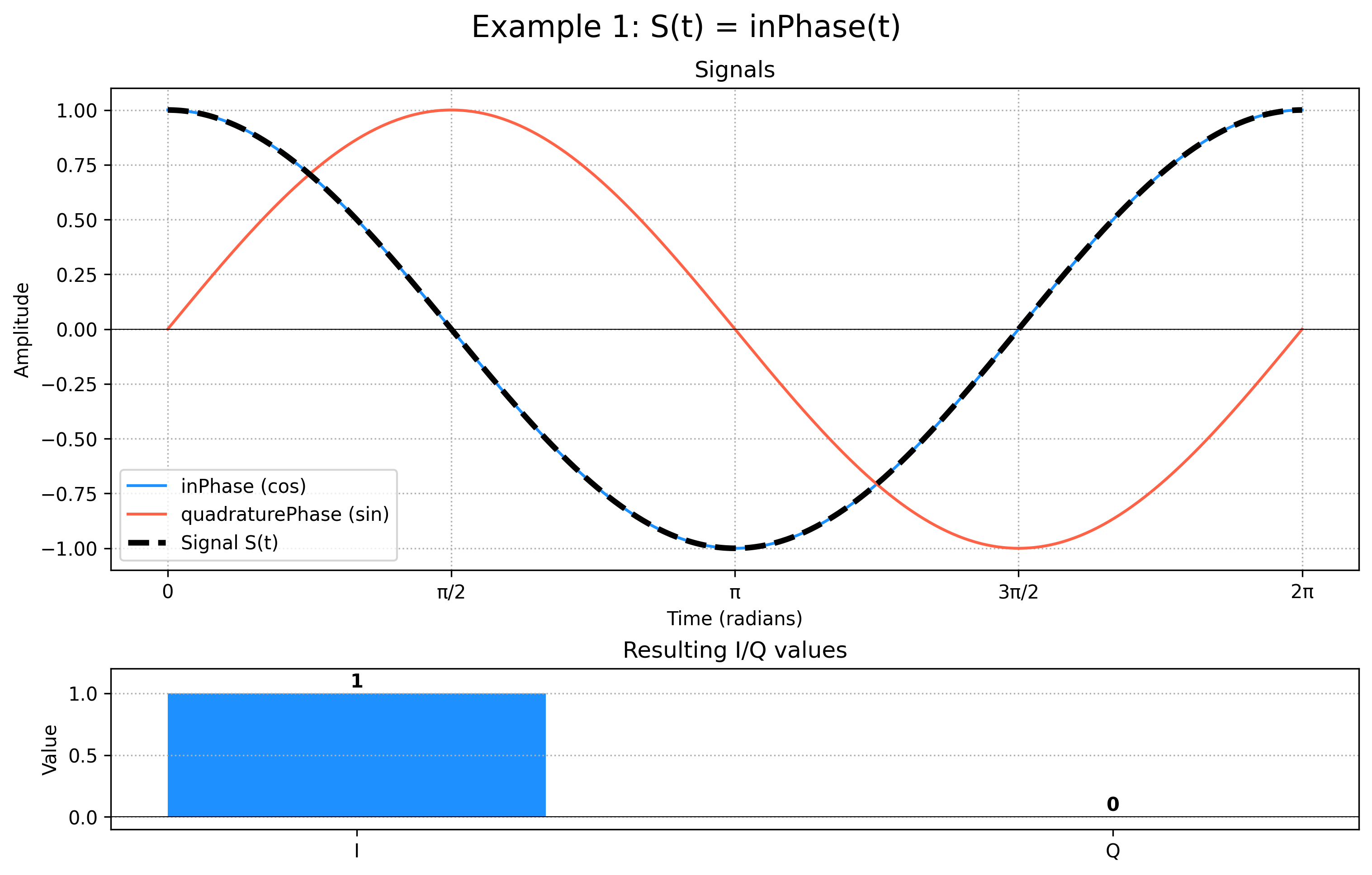 Signal example 1
In this example,S(t)=inPhase(t), so in the context ofI×inPhase(t)-Q×quadraturePhase(t),I=1andQ=0.
📝 Example: The case where S(t) is a sine wave like the in-phase signal, except it "leads" the in-phase signal by 90°. Relative to the in-phase signal, the phase of S(t) is 90° (orπ/2, in radians).
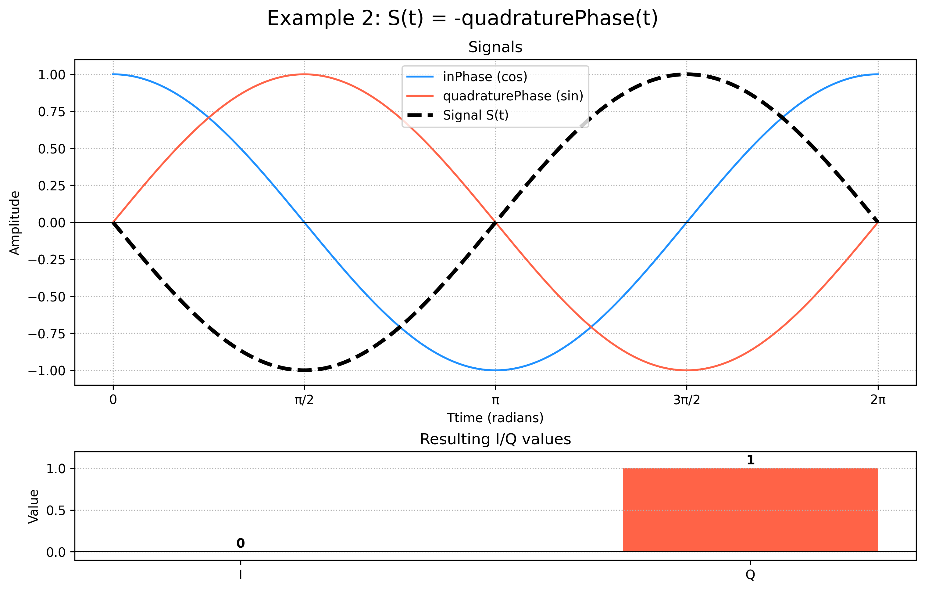 Signal example 2
In that example,S(t)=-quadraturePhase(t)(note the minus sign, since S(t) "leads" the in-phase signal, while the quadrature-phase "lags" behind the in-phase signal), so in the context ofI×inPhase(t)-Q×quadraturePhase(t),I=0andQ=1.
We can imagine[I,Q]being a vector in the plane (with I being associated to the horizontal axis). Looking at these two examples, we see that the angle of the vector [I,Q] (relative to the horizontal axis) represents the phase of S(t), while its length represents the amplitude:
- In the first example, I=1 and Q=0, so the angle of [I,Q] is 0, which corresponds to the phase of S(t). The amplitude is 1, which also corresponds to the amplitude of S(t).
- In the second example, I=0 and Q=1, so the angle of [I,Q] is 90°, which corresponds to the phase of S(t). The amplitude is 1, which also corresponds to the amplitude of S(t).
Based on these two simple examples, we have an intuition for the rule. It turns out that this generalizes to any amplitude and phase. This vector representation of[I,Q]on the plane is called the phasor diagram.
🔍Closer look: The math behind IQ samplingLet us consider a radio sine wave at amplitudeA, frequencyFand phaseP, denotedS(t)=Acos(2πFt+P)Assume that the SDR is "tuned" at the frequencyF. The in-phase signal iscos(2πFt)and the quadrature-phase signal issin(2πFt).
Then we haveS(t)=Icos(2πFt)-Qsin(2πFt). Let us compute theIandQvalues for each sample to relate them to S(t)'s amplitude and phase.
By using the cosine addition formula, we see that:
Acos(P)cos(2πFt)-Asin(P)sin(2πFt)=Acos(2πFt+P)
ThereforeI=Acos(P)andQ=Asin(P), so the phase isarctan(Q/I)and the amplitude isI2+Q2
As we see, a radio sine wave at exactly the same frequency as the SDR tuning frequency will be represented by a constant vector, whose angle and length represents the phase and amplitude of the sine wave.
But what happens if our radio wave is a sine wave not exactly at the SDR tuned frequency? Let's say that our radio wave is a sine at frequencyF+δ. The intuition here is that a shift in frequency can be thought of as a phase variation. Indeed, our phasor will "spin" in the positive (counter-clockwise) direction at a rate ofδturns per second like this:
 Phasor spinning
Conversely, if the radio wave frequency is less than the SDR tuning frequency, the phasor will "spin" in the negative direction, with a speed proportional to the frequency difference.
🔍Closer look: Frequency and phase-variation equivalenceLet us express our radio waveS(t)=Acos(2π(F+δ)t)which can also be writtenS(t)=Acos(2πFt+2πδt), where the term2πδtcan be thought of as a phase.Therefore,S(t)can be thought of as a sine wave of frequencyF, but with a phase that varies in time at a rate ofδturns per second.
Now, we see that the IQ samples (and the phasor) contain all the information we need about the signal:
- Its phase (the angle of the vector relative to the horizontal axis)
- Its amplitude (the length of the vector)
- Its relative frequency to the SDR tuned frequency (the "spinning" speed)
Filtering
The SDR can capture a wide range of frequencies around its center frequency. When listening to a specific signal, we will tune our SDR to the frequency of this signal, but other signals may be present in the captured frequency range, polluting our data.
For this reason, we usually apply a low-pass filter to our IQ data to keep only the signals around the center frequency (we use a low-pass filter and not a pass-band filter, because recall that due to IQ sampling, a signal with the exact same frequency as the SDR center frequency will appear in the IQ data as a frequency of 0, i.e., a DC offset).
The low-pass filter is some kind of moving-average on the IQ data that smoothes out the fast variations (corresponding to signals too distant from our center frequency) and keeps the signal that we need to focus on.
🔍Closer look: Real-world filteringThe "moving average" analogy is a simplification. In reality, a filter is a convolution operation, which is a sort of weighted moving average. The weights, called the filter taps, determine its precise characteristics. Filtering is used for mainly two reasons:- Channel filtering: This is the role we described above (isolating our signal). The key parameter is the cutoff frequency, which defines the boundary between frequencies to keep (the low frequencies in IQ signal, corresponding to the band around the SDR tuning frequency) and high frequencies to reject. A good filter has a sharp transition between the two to effectively cut out adjacent signals without distorting the one we want.
- Pulse shaping and Matched Filtering: In digital communications, we also filter to prevent Intersymbol Interference (ISI). This happens when the signal from one symbol "blurs" into the next, making it hard for the receiver to decide which symbol was sent.
📝 Example: Filtering IQ signal
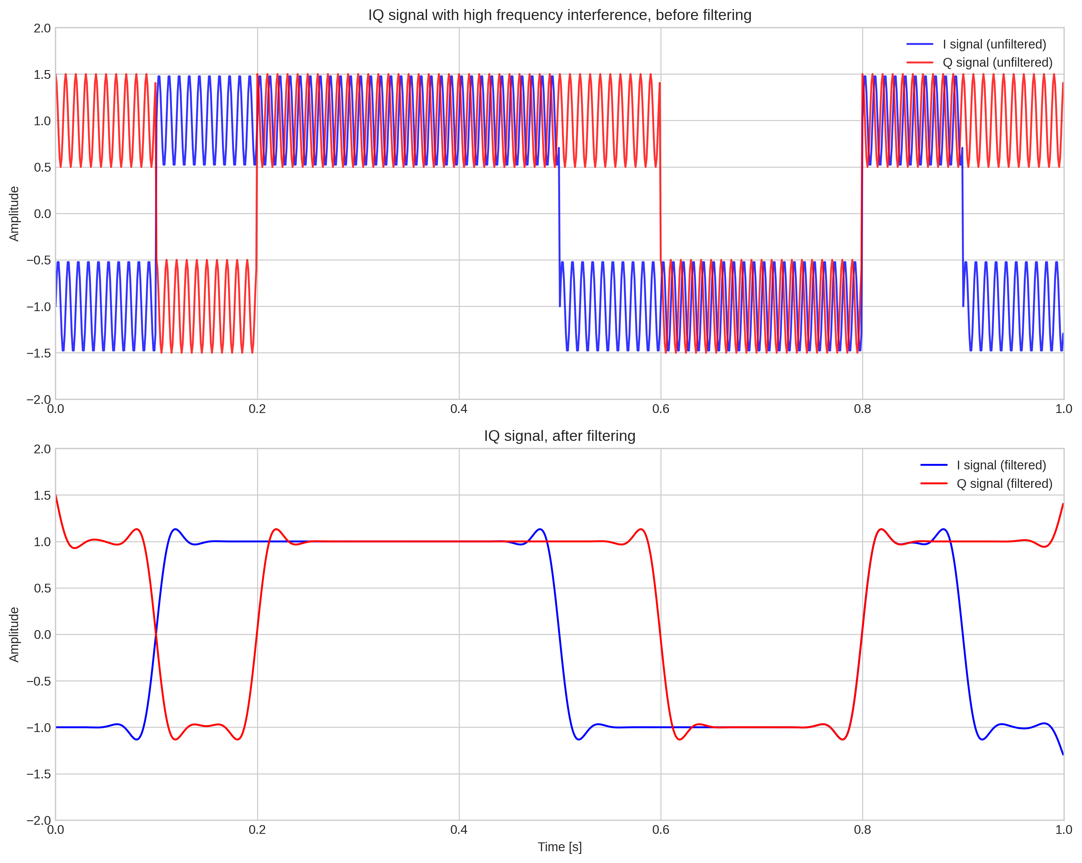 Filtering IQ signal
Listening on multiple channels simultaneously (aka: the "Super-power" of the SDR)
We have already seen that the SDR listens to a wide range of frequencies around its center frequency. This is why we need filtering to eliminate other conflicting signals in the frequency range.
But what if that could be used to our advantage? During BLE sniffing, due to channel hopping, it would be useful to be able to listen to multiple Bluetooth channels simultaneously. It turns out that this is possible, as long as all the channels are in the correct frequency range around the center frequency.
Suppose our SDR is tuned to the frequency of 1000Hz (this is not a realistic value, but it is used in our example for the sake of simplicity). We record some IQ data, and we know that on this data there is a signal at 1001Hz.
How do we listen to this 1001Hz signal without having to physically tune the SDR at 1001Hz? We will need to post-process our IQ data to get IQ data similar to what would have been obtained if the SDR was tuned at 1001Hz.
Recall that, because the signal is at 1001Hz and our tuned frequency is at 1000Hz, the phasor obtained from the IQ data will "spin" at a rate of 1 turn per second in the positive direction (counter-clockwise).
What would have been the phasor if the SDR was tuned to 1001Hz? It would be a constant vector. Therefore, to perform this kind of "software tuning", we will need to take our raw IQ data and apply a time-variant rotation of 1 turn per second in the negative direction (clockwise). This corresponds to a frequency shift. The resulting IQ data will be similar to the data we would have obtained if the SDR was tuned to 1001Hz.
In a nutshell, we "correct" in software the phasor rotation caused by the frequency difference to obtain a stable phasor as we would have obtained if we were tuned precisely to its frequency. Only then can we apply the low-pass filter.
By this process, we see that from the same recorded IQ data, we can extract signals at various frequencies around our center frequency by:
- Applying a frequency shift to the data to "center" around our target signal
- Applying a low-pass filter
Demodulation
The BLE protocol employs GFSK (Gaussian Frequency Shift Keying) modulation, which is a kind of frequency modulation. Bits are transmitted at a fixed rate of 1 MHz, and the signal frequency determines the value of the bit: a signal frequency higher than the central frequency represents a 1, while a lower frequency represents a 0.
In order to demodulate the signal (i.e., extract the 0s and 1s from the IQ data), we will first need to recover the frequency of the signal at each point in time. Recall that the frequency is simply the phase variation, so to compute the frequency at time T, we will need to compare (subtract) the phase at time T and at time T+1.
📝 Example: Demodulation
The following figure shows the demodulation of a simple signal.
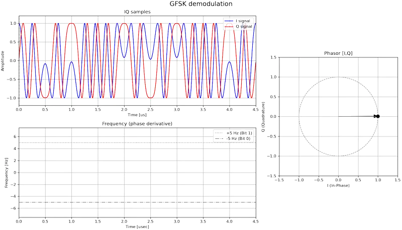 Demodulation example
We can see that to have a clear demodulation, we will need to sample the frequency curve precisely at the center of each bit. In order to find out precisely the centers of the bits, we will use the preamble. The general idea is to pre-compute an ideal preamble template and find out at which point in time the preamble template is the most similar possible to our incoming signal.
📝 Example: Preamble detection
The following figure shows this process, we see that the maximum correlation is at the actual preamble start, at T=6.
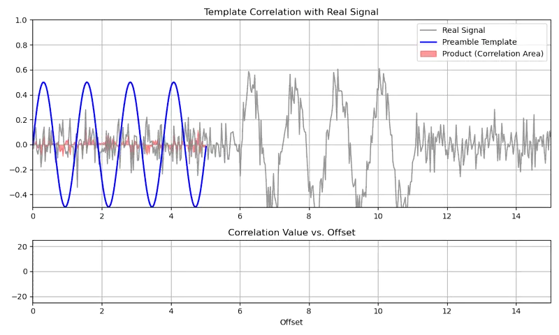 Animation showing preamble correlation
Once this is done, we can decode each bit by looking at the frequency at the center of the symbol.
🔍Closer look: Preamble and synchronization in practiceThe signal in the above example is nicely normalized, but it is rarely the case in practice. That's why we usually do a normalized cross-correlation. The normalized cross-correlation normalizes each signal by subtracting its mean, and dividing by its standard deviation.Furthermore, a Phase-Locked Loop (PLL) could be used to achieve precise symbol timing synchronization and account for clock drift. The PLL continuously adjusts the receiver’s sampling instant to lock onto the exact centers of symbols, using a feedback that measures timing error. It tracks and corrects small drifts caused, for example, by clock mismatches.
The HackRF One is a popular and affordable open-source SDR device. Its key appeal lies in its wide frequency range and its completely open-source design, covering both the hardware and the firmware. This openness allows researchers to not only use the device for a vast range of applications, but also to modify its firmware to implement custom features, a capability we leverage heavily in our approach.
The HackRF can listen to signals in frequencies from 1 MHz to 6 GHz, but works best in the range 2 GHz-2.8 GHz, which is great because the BLE frequencies are in it.
The IQ sampling rate and maximum bandwidth is 20 MHz. This means that we can listen simultaneously to multiple signals around our center frequency, from [center - 10 MHz] to [center + 10 MHz].
There are three RX gain parameters that can be modified: RF, LNA, and VGA gain. The RF and LNA gain operate right after the signal is received, but the VGA gain operates after converting the signal to IQ, just before the sampling.
Later in this post, we will see how we implemented the AGC (Automatic Gain Control) in the HackRF firmware.
The HackRF interacts with the Host using a USB interface. There is a USB endpoint to perform control operations (such as setup, setting frequency, gain, and so on), and two bulk USB endpoints to carry respectively received and transmitted IQ samples.
The HackRF employs an ARM processor with two cores, M0 and M4. The M0 core is dedicated to handling the IQ data flow. It spends its time moving IQ data between the transceiver and a shared buffer with the M4. The M4 core runs the rest of the firmware.
The HackRF uses a MAX5684 Analog Front-End and sends commands to it with SPI.
While the theory of BLE and SDRs provides a solid foundation, applying it to real-world sniffing presents a number of practical challenges that can quickly derail any attempt to capture a full communication. These problems stem from the physical realities of radio transmission, the performance limitations of a host-controlled SDR, and the stateful nature of the BLE protocol itself. In the following sections, we will detail the three main obstacles we needed to overcome.
Near/far effects
When sniffing the BLE connection between a central and peripheral devices, transmit power can vary a lot: the signal strength from the central device may be high, while the signal strength from the peripheral device may be low.
Setting a low gain will enable capturing the packets from the phone correctly, but the packets from the peripheral devices will have an insufficient signal strength. Conversely, if we set a high gain, we will be able to correctly capture peripheral device packets, but phone packets will be clipped/distorted, impairing the demodulation process.
Attempting to adjust the gain once the beginning of the packet is received using the USB interface will be too slow, due to the USB command latency.
Channel switching latency
The BLE protocol employs channel hopping at a fast rate. Attempting to follow the channel hopping from the host by sending commands to the HackRF via the USB interface would be too slow, again due to the USB command latency.
Sniffing advertisement channels
The BLE advertising channels are 37, 38, and 39. The frequencies of these channels are too far apart (> 20 MHz) for HackRF to be able to listen to more than one of them at the same time. Since the CONNECT_IND packet can happen on any of the advertising channels, we will probably miss it and fail to catch the required parameters (notably, the Access Address that is required to compute the channel hopping).
This section present the solutions to three challenges we encountered.
Firmware-based Automatic Gain Control (AGC)
The disparity in signal strength was tackled by the implementation of an Automatic Gain Control (AGC) to automatically adjust the input gain based on signal strength. In order to have a fast AGC, it needed to be implemented in the time-critical receive loop of the HackRF's firmware, thus entirely bypassing the high-latency USB connection.
Unlike traditional continuous AGCs that constantly adapt the gain based on signal power, this implementation uses a one-shot approach triggered only when a packet is detected.
The reason is simple: if the AGC keeps running during idle periods, it ends up amplifying noise, which leads to saturation and clipping as soon as a real packet arrives. Once the receiver is clipped, it’s impossible to estimate the correct gain in time for decoding. By freezing the gain during idle and only adjusting it at the start of a packet, the AGC can directly compute and apply the correct gain level so that the signal is stable as soon as possible.
Let's now focus on the implementation details, by diving into the firmware function that handles the receiving mode:
This code runs on the M4 core, but the usb_bulk_buffer buffer and m0_state struct are shared with the M0 core. The M0 core fills up the buffer by blocks of 32 bytes at a time, and increments m0_state.m0_count accordingly. When there is sufficient data (USB_TRANSFER_SIZE) the data is sent to the host via USB bulk transfer.
In order to have a fast AGC, it needs to be implemented in this loop, and executed on the M4 core. It cannot be executed on the M0 core since this core is too much time-constrained to be able to do any other thing besides copying IQ data.
The AGC will need to start as fast as possible, so we will need to process each 32-byte block and feed it to the AGC function, so we insert this code at the start of our while loop:
The auto_gain_control function repeats this process for each received packet:
- Sets the VGA gain to a baseline (low) value.
- Detect idle noise power level, and track it using a rolling average
- When there is an increase in power such that the SNR is over a defined threshold, detects the start of a packet.
- Measure the power at the start of the packet, and use it to compute the optimal VGA gain
- Apply the computed VGA gain, and update the noise power level under that new gain.
- When the SNR falls under a defined threshold, detects the end of a packet, and reset the VGA gain to the baseline value.
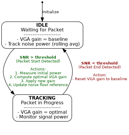 AGC state machine
In order to make the AGC more reactive, we also increased the SPI clock frequency in the HackRF firmware. The following picture shows the effect of the AGC, increasing the power when a packet is detected. The AGC takes effect a little after the beginning of the preamble, leaving ample opportunity to decode the packet.
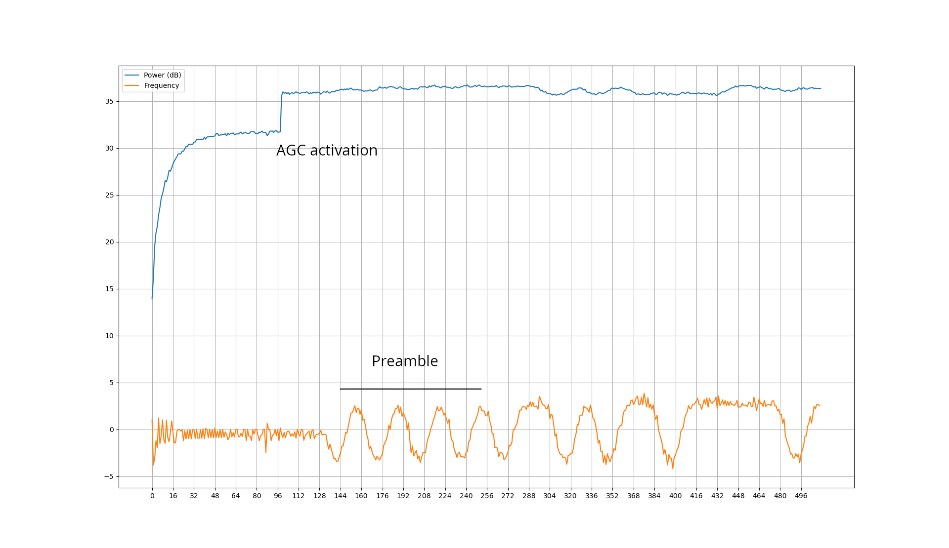 AGC effect on a received BLE packet
This firmware-implemented AGC significantly improves the signal power range of packets that can be detected and processed correctly.
Frequency change scheduling
In order to follow the BLE channel hopping, the frequency change command using the USB interface will not do, due to USB latency and jitter. We also can't implement the whole channel hopping algorithm into the firmware due to performance constraints.
Fortunately, the host that implements the BLE channel hopping knows in advance when to change the frequency. The solution is to implement a scheduled frequency change USB command that allows the host to tell the HackRF to change the frequency at a specific sample. This way, the host can schedule in advance the frequency changes necessary for BLE channel hopping.
This will have to be implemented in firmware, in the same rx_mode() function as the AGC.
First, we will have to implement an USB command to allow the host to schedule a frequency change:
Then we will need to add this to the rx_mode() loop:
With this new USB command, the HackRF One acquires the capability of executing frequency changes at precise, future sample counts.
Deducing channel hopping state
In our typical use case, we want to sniff an established BLE connection without having captured the CONNECT_IND packet. This is due to two reasons:
- We may start the sniffing process as the connection is already established
- The HackRF bandwidth does not allow us to listen simultaneously on all advertising channels, so there is a high probability that we will miss the CONNECT_IND packet even if we started the sniffing process before the connection is established.
Recall that the channel is changed at each connection event, and that the time between two connection events is called the connection interval. The channel used for a specific connection event depends on three parameters:
- The Channel Map, also sent in the CONNECT_IND packet, specifying the set of data channels in use on this connection. For the sake of simplicity, we will consider that the connection uses all data channels, which is a realistic hypothesis.
- The Access Address of the connection (sent in the CONNECT_IND packet)
- The connection event counter (i.e., the number of connection events from the start of the connection, before the current connection event)
The Access Address follows the preamble in each data packet, so it can be sniffed once we capture any packet belonging to the connection. However, the connection event counter is a hidden state (known by the central and peripheral devices) that is never sent, and must be deduced.
Our approach is based on a process of elimination, similar to a sieve. The general idea to deduce the counter is to listen on a wide number of channels (the HackRF, given its bandwidth, can listen simultaneously on 6 data channels) and try to sniff connection events. We begin with the entire space of65536possible counter states, each observed packet acts as an oracle, enabling us to eliminate a large number of incorrect states.
Each time we observe a connection event, based on the channel and time at which the connection event was observed, we remove from the set each counter value that is incompatible with this observation. We repeat the process until there is only one value in the set.
Once this value is known, we can follow precisely the channel hopping of the BLE connection.
📝 Example: Recovering the counter value
Let's say that we observe the start of a connection event at time T=0μsec on channel 1, and that the connection interval is45000μsec. Sniffing the connection event also allows us to get the access address. Given the access address, we can fully determine the channel based on the counter.
Now, let's try to narrow down the possible counter values for this connection event:
- Assuming a counter value of 0, the channel is 5 (incompatible)
- Assuming a counter value of 1, the channel is 15 (incompatible)
- Assuming a counter value of 2, the channel is 1 (compatibe!)
- Assuming a counter value of 3, the channel is 23 (incompatible)
- Assuming a counter value of 4, the channel is 1 (compatible!)
- Assuming a counter value of 5, the channel is 9 (incompatible)
- ... and so on.
Now, we know that the counter value for this connection event is certainly not 0, 1, 3, or 5 (and so on). The set of possible counter values is refined as:S={2,4,...}
Let's assume that we observe the next connection event atT=90000μsec on channel 4. Based on the time elapsed since our previous observed connection event, we can say thatcurrentCounter-previousCounter=90000/connInterval=2. Indeed, that means that between our two observed connection events, another connection event occurred (and was probably missed because it was outside our frequency range). For the needs of our example, let us suppose that this missed connection event occurred on channel 7:
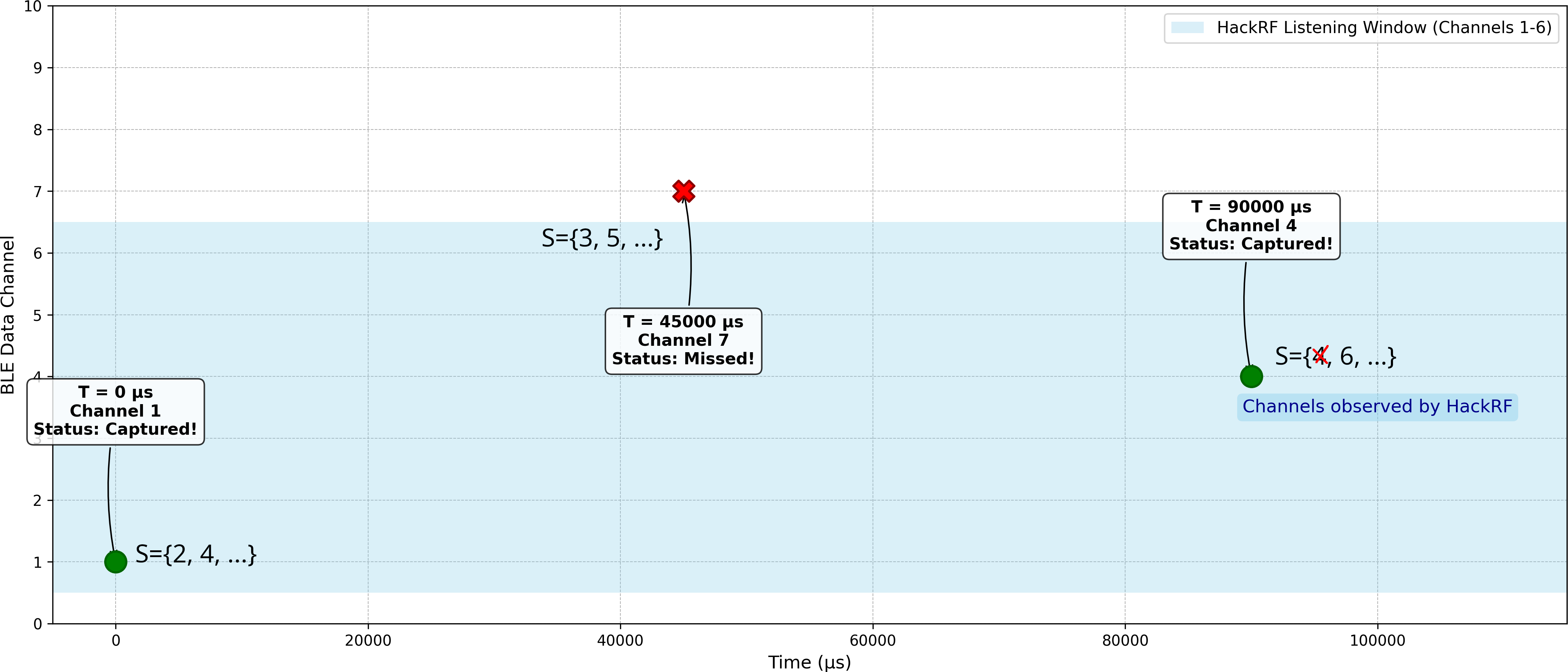 BLE channel hopping
It means that, based only on the information gathered from the previous connection event, the set of possible counter values for the current connection event is{s+2|s∈S}={4,6,...}
Now, let us refine again our set of possible values:
- Assuming a counter value of 4, the channel is 29 (incompatible)
- Assuming a counter value of 6, the channel is 4 (compatible!)
- .. and so on.
We have successfully eliminated4from the current possible counter value set, and the set is now{6,...}
This process is repeated until there is only one value in the set.
To demonstrate this approach, we will configure a BLE Peripheral device on a phone and a BLE Central device on a laptop.
Peripheral device setup
For the BLE Peripheral device, we need to install nRF Connect on an Android phone, then configure an advertiser and a GATT server with a readable characteristic.
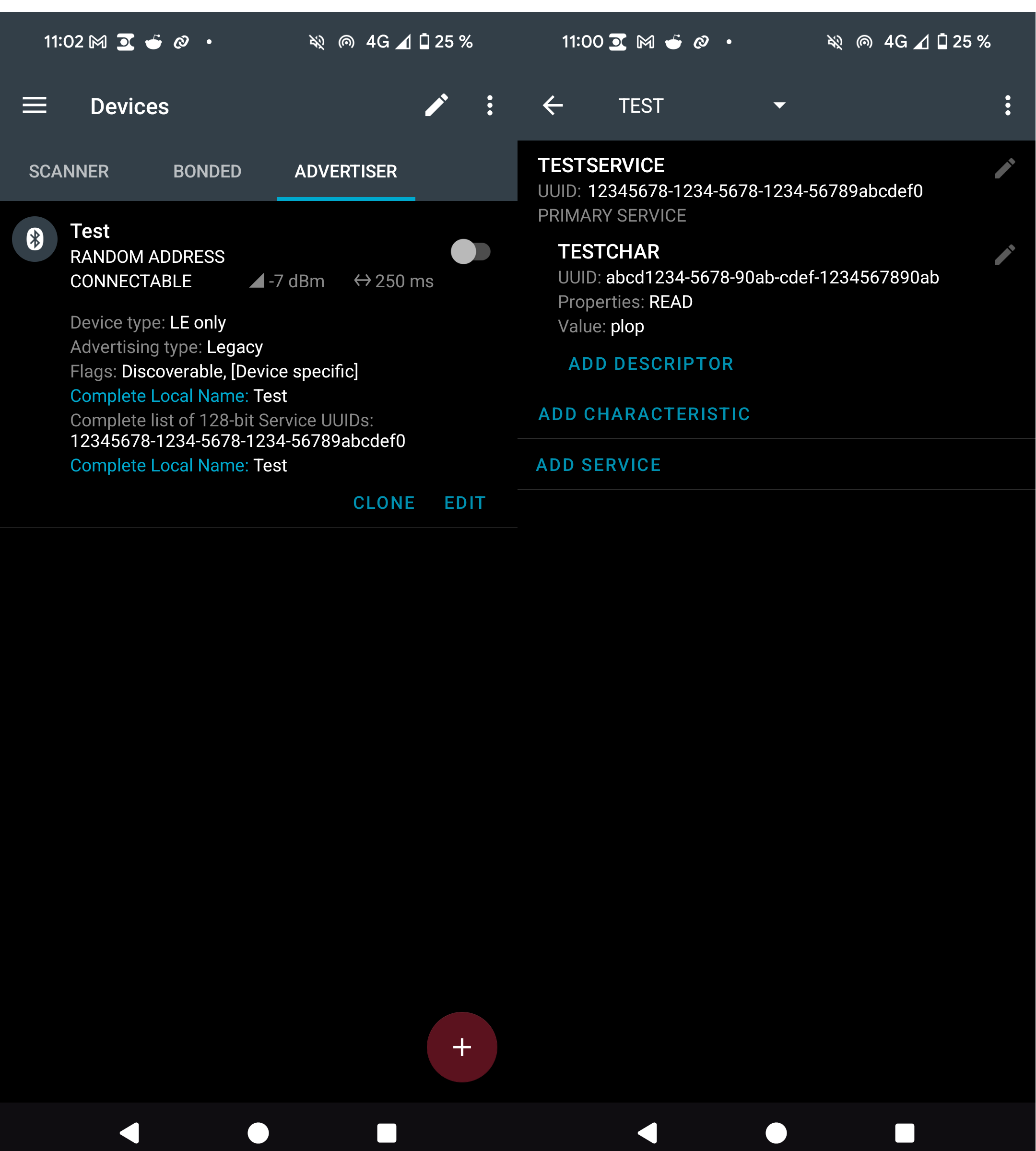 nRF Connect configuration
Central device setup
The BLE Central device is a laptop using the Python bleak module.
The BLE physical layer supports multiple modes:
- 1M PHY
- 2M PHY
- Coded PHY
Our tool supports only 1M PHY for now, so we will need to use btmgmt to force the use of this mode:
Then, we will need a sample client Python program (using the bleak Python module) to connect to our server:
Intercepting the connection
First, we launch the BLE Client (we can detect the MAC address by doing a scan with any tool):
Once the connection is established, we launch our tool to sniff the connection:
The arguments are:
- -p capture.pcap: Capture L2CAP data packets to a pcap file
- -w samples: Record IQ samples to a file
- -c 5: Set the main listening channel to 5
- -b: Enable HackRF RF amp
- -l 30: Set LNA gain to 30
- -g 10: Set VGA gain to 10
- -W 6: Also listen on 6 channels around the main channel (i.e., channels 2, 3, 4, 6, 7, 8 in addition to 5) while resolving counter init value
- -o: Enable connection tracking / channel hopping
- -v -d: Enable verbose and debug output
- -A: Enable AGC in the firmware
It is also possible to specify the Access Address corresponding to the connection we want to sniff using the -a option. If it is omitted, the tool will try to guess the Access Address and sniff the first connection available.
Here is a demo video showing the tool in action: it sniffs channels from 2 to 8, quickly recovers the channel hopping counter value, and tracks the connection (the only option that was added for the demo is the -a due to the noisy test environment):
The resulting packets are written to the pcap capture file, which can be opened in Wireshark:
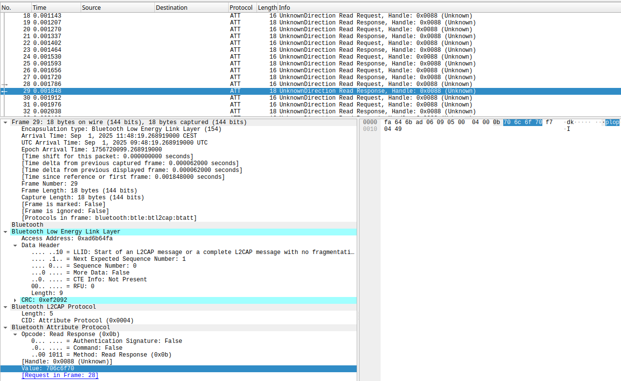 Wireshark showing BLE packets
In this post, we have detailed a complete methodology for sniffing BLE connections using a HackRF One, overcoming the significant challenges of near/far power disparities, channel hopping latency, and missing initial connection parameters. By modifying the HackRF firmware to implement a fast AGC and a scheduled frequency change mechanism, and by using a logical process to deduce the connection state, we transformed a general-purpose SDR into a powerful, specialized BLE analysis tool.
Discussion on strengths and limitations
The approach to recover the hopping state by observing packets of an existing connection is not new, it has been done in the excellent BTLEJACK approach by Damien Cauquil, using hardware (non-SDR) radio. In this blog post, we replicated some of the BTLEJACK features using a software-defined radio.
Using an SDR to perform this approach has a number of advantages:
The SDR is able to sniff multiple channels at once (in our experience with HackRF, we were able to sniff up to 7 BLE channels simultaneously before running into signal quality problems). This greatly reduces the length of the hopping state recovery phase, since we are able to sniff more packets (the video demo shows that it takes 1 to 2 seconds to lock onto a connection). This also helps with managing the clock drift since the time between two packet captures will be smaller.
Since all the signal processing is implemented in software, it is easy to add support for new versions of the BLE specifications (for example, new PHYs) without having to modify the hardware.
Despite this, we acknowledge the following limitations, some of them could be mitigated by future work:
The most prominent limitation is the incompressible time delay for reacting to a signal and applying the gain. Even if doing it in the firmware is very fast compared to doing it on the host via USB, it is still several dozen microseconds. Since the AGC needs to react very fast, it limits the number of gain changes that can be done and limits the acceptable range in signal power. This makes our approach less reliable if there is a large disparity in signal power between both ends of the sniffed connection. This limitation could be worked around by implementing a more specialized and sophisticated AGC that remembers previous packets from the same device (for example, using timing properties) and their power.
Another timing limitation is the time delay for switching frequencies, even in the firmware. Since the HackRF One can listen to multiple channels simultaneously, it would be interesting to exploit that fact to reduce the occurrences of frequency switching during the connection tracking phase. Since the channel hopping schedule can be known in advance once the counter value is recovered, one could compute a schedule that minimizes the number of frequency switches while allowing the bandwidth of the HackRF One to cover all the needed channels.
The tool supports only LE 1M PHY and the new channel selection algorithm (CSA#2), and does not support connection interval or channel map recovery. These features could be implemented in the future.
Perspectives
The capabilities developed here open the door to more advanced security research beyond passive sniffing. The precise timing and control achieved are foundational for active interactions. For instance, one could build upon this work to inject custom packets into an established connection, perform man-in-the-middle attacks, or implement highly targeted jamming to disrupt specific communications selectively. This demonstrates the immense power and flexibility that open-source hardware and firmware provide, enabling researchers to build sophisticated tools tailored to complex security challenges.

