Time Series Forecasting with Graph Transformers

Time series forecasting is a cornerstone in modern business analytics, whether it is concerned with anticipating market trends, user behavior, optimizing resource allocation, or planning for future growth. As such, a wide range of different approaches have been introduced and investigated for forecasting, lately data-driven approaches using machine learning and generative models.

This blog post will dive into forecasting on graph structured entities, e.g., as obtained from a relational database, utilizing not only the individual time series as signal but also related information. As most of the world’s data is stored in relational structures, this topic is of particular interest for real world applications. We describe an end-to-end pipeline to perform forecasting using graph transformers and specifically discuss predictive vs. generative paradigms.

Forecasting on Graph-structured Data

Forecasting is the process of making predictions about future events based on historical data and current observations, requiring detecting patterns, trends, and seasonal variations.

Traditional forecasting methods often treat time series data in isolation, focusing solely on temporal patterns within a single sequence. However, in real-world applications, valuable predictive signals often exist in related data sources. For instance, when forecasting product sales, factors such as marketing campaigns, competitor pricing, or regional economic indicators can significantly impact the accuracy of predictions. Graphs are a natural structure to represent such inter-connected data sources. They represent a set of inter-connected nodes of different entities, where some entities can have time series that can be forecasted. Each node can potentially hold a variety of features that hold important signal for forecasting tasks on other nodes. Further, they lend themselves to a wide arrange of machine learning methods, e.g., Graph Transformers.

A prominent option for obtaining graphs directly from an underlying business problem on a relational database is Relational Deep Learning (RDL), which automatically discovers and utilizes cross-table relationships and data in connected tables. The RDL scheme allows to automatically extract a graph structure from the relational database, allowing us to treat timeseries forecasting as a graph learning task. We will use the graph obtained via RDL as an example below. However, our graph forecasting techniques are not limited to graphs obtained via RDL but can be applied on arbitrary forecasting tasks where time series have to be forecasted for a subset of graph nodes.

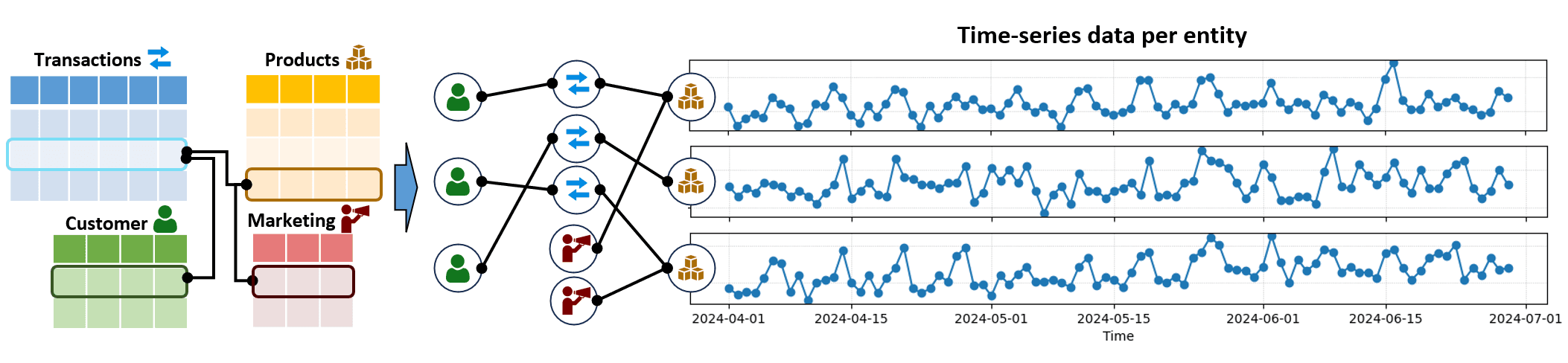
Example. Consider the task of forecasting the sales per day for all products stored in a product table (yellow). Further tables containing transactions (blue), customers (green), product marketing (red) can provide additional signals that help solving the task. Using the RDL scheme, we can automatically transform the relational tables into a graph with node features. Then, the task is to perform forecasting on the subset of product nodes via graph machine learning.

Notation. We denote the input to our graph forecasting task as a graph with node set and edge set , where is a subset of nodes that serve as forecasting entities with a given (past) time series . Additionally, the graph nodes are annotated with arbitrary node features , e.g., encoded row features.

Core Forecasting Framework

We formulate the core forecasting framework for a single time series of an entity as

where a function predicts or generates the next time series value given a set of conditioning signals , , , and . The function , e.g., modeled by a Multi-Layer Perceptron (MLP), is shared over all . The conditioning signals serve specific purposes as follows.

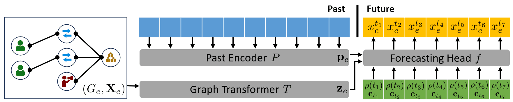
Architecture Overview. Data flow shown for one entity. The forecasting head unifies information from the graph, the past time series, temporal frequency encodings and calendar features. While past and graph encodings are given for the whole entity, the temporal encodings and calendar features are individual for each future prediction.

Date-time encodings. To provide the model with information about the current date, current time, day of week, month of year, etc, frequency encodings of several date-time values are provided to the model. Date-time encodings enable to correctly model seasonal effects.

Calendar encodings. Embeddings represent indicators given in calendar tables. These can be indicators for specific holidays or other special times, which could be relevant for the model. We find that providing such information explicitly improves the models ability to capture, e.g., rare outlier days with specific characteristics. Embeddings are processed by a 1-dimensional CNN before fed into to allow the model to see a window of adjacent calendar information.

Graph entity encodings. Embeddings encode the subgraph around entity e obtained via temporal subgraph sampling according to the RDL formula. After neighbor sampling, the embeddings can be obtained with a graph transformer or graph neural network on and , as described in a dedicated section below. The entity subgraph conditioning allows the model to consider rich signals occurring in relational data.

Past sequence encodings. Auto-regressive signals are important for any forecasting model. Thus, the past time series for entity is encoded into embedding with a sequence encoder, e.g., a Transformer, and provided to the model. The past sequence encoding allows the model to react to the current trend in the time series. We describe the past encoders in a dedicated section below.

Graph Encoding via Graph Transformers

The forecasting head is conditioned on node embeddings for each entity , respectively. A temporal neighbor sampler can be used to obtain subgraphs with features around entities , allowing to scale the approach to real world graphs. If temporal graphs are present (such as in the RDL context), subgraphs are sampled to only contain nodes with a timestamp smaller than current time , preventing data leakage from future information in the given graph. The subgraph can then be encoded with a Graph Transformer:

Graph Transformers employ graph positional encodings of the given graph , which allow a sequence Transformer architecture to process and understand the graph structure underlying individual node features . For an in-depth discussion about Graph Transformers, check out our Graph Transformer blog post.

Past Sequence Encoder

The past embedding is another important conditioning for function . Auto-regressive models have been shown to perform well in forecasting tasks, allowing the model to continue current trends in recently observed past values. To this end, we encode the past sequence for each entity with a past encoding network:

In theory, any sequence encoder can be used, such as transformers, convolutional neural networks (CNNs), or simple MLPs. We found that one-dimensional CNNs performing convolution over the temporal dimension provide a good trade-off between efficiency and accuracy.

Training

The above forecasting framework provides a deep learning architecture that can be trained in an end-to-end fashion on existing graphs with time series per entity. Naively, we can sample a specific time , apply temporal sampling to sample subgraphs with timestamp earlier than and train the network to predict future values at time by minimizing an MSE loss against ground truth time series values :

Regression vs. Generative Forecasting

At its core, time series forecasting is a probabilistic task due to ambiguities in the mapping from input signals/features to future value. Thus, it is reasonable to consider a more advanced framework than above, where we model distributions over random variables instead of a function:

Here, it is assumed that the future value follows some conditional distribution, from which we can obtain the most likely value or perform probabilistic inference via sampling.

Forecasting via Regression. In the above framework, the function is naively modeled with an Multi-Layer Perceptron (MLP) and trained to regress value by minimizing a mean-squared error. This paradigm provides good forecast in an efficient manner. However, simple regression via MSE implicitly assumes to be Gaussian and trains the model to predict the mean of that Gaussian, which is a conceptual limitation of the given framework. A result is that the naive regression head above is prone to mean collapse, potentially smoothing out higher frequency forecasts, especially if the actual distribution is far away from a Gaussian, e.g., multi-modal.

In the past, forecasting research came up with alternatives, e.g., optimizing the negative log likelihood of examples given a parameterized distribution, with distribution parameters predicted by the model. This allows to predict the full distribution instead of individual point estimates and provides additional outputs, such as quantile bands as a measure of uncertainty. Typically, this is used to model Gaussian distributions or alternatives for discrete forecasts like the Negative Binomial distribution. However, one crucial limitation remains: the given time series data needs to follow a parameterized distribution in the first place and that distribution needs to be assumed a priori.

Generative Forecasting. Here, we explore an alternative probabilistic inference formulation based on recent research in continuous generative modeling, concretely, conditional diffusion models. Instead of using a simple regression MLP , we use a diffusion head, which iteratively denoises a randomly initialized future time series, conditioned on the embeddings from above.

The diffusion head, modeled via a CNN, takes above conditionings , , and iteratively denoises a noisy time-series. During training, we follow the common practice of a Denoising Diffusion Probabilistic Model (DDPM) schedule over 1000 steps, adding noise to a future time series and training the model to predict the added noise. During inference, we start with a time-series randomly initialized from a Gaussian distribution and iteratively denoise it until obtaining a sample from the modeled distribution.

Modeling the time series forecasting task in this manner enables some interesting properties. Firstly, the trained model allows to sample values from without making any assumption on the form of . We can sample multiple times and statistics can be obtained empirically, by extracting modes or providing quantile bands. We can obtain an empirical mean and variance, which would require again the assumption on the distribution type. However, we can also empirically extract modes or provide quantiles bands.

Forecasting Results

In the following, we provide some example forecast for a task of predicting future visits in individual stores. We observe that the generative model is able to forecast higher frequency details and reacts better to rare events than the predictive forecasting baseline. In quantitative comparison both perform equally well, though.

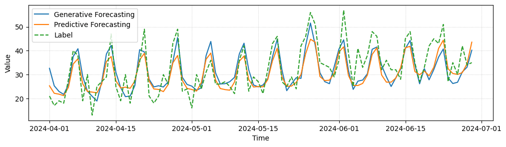
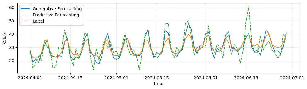
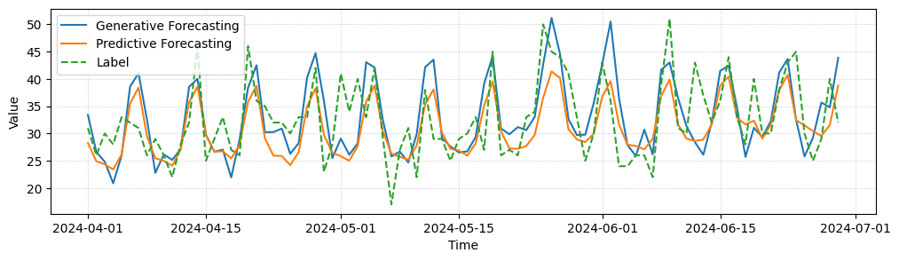
Generative Forecasting Comparison. We compare predictive and generative forecasting results for three entities of a forecasting task, where our models make one prediction per day for the next 90 days in advance. While quantitatively both models perform similarly well, generative forecasting shows less mean collapse and captures some high frequency details better.

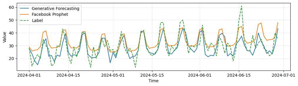
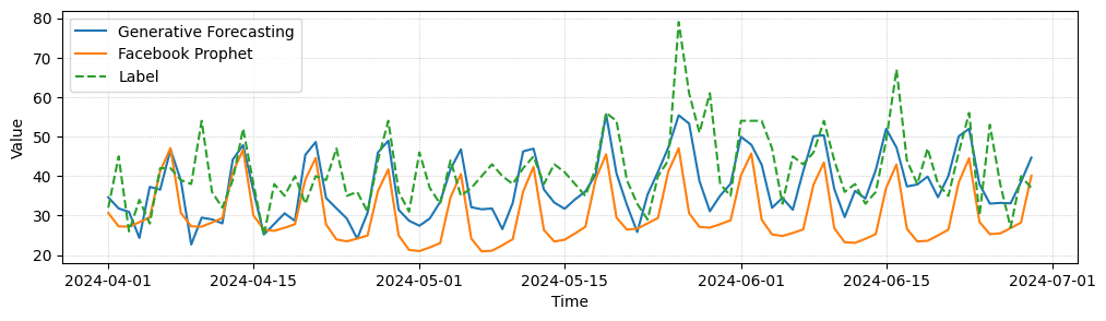
Comparison to Facebook Prophet. We compare our forecasting results against forecasts from Facebook Prophet. While Prophet also captures trend and seasonality mostly correct, it shows slightly more divergence and more mean collapse behavior.

Conclusion

Time series forecasting has been and will continue to be an important task in machine learning for several different applications. In this blog post, we described how to design an end-to-end pipeline for forecasting on graph structures, performing forecasting on a subset of graph nodes while using input signals from the whole graph, e.g., to combine data from multiple tables in a database. We also discussed the differences between point predictions and probabilistic forecasting using generative formulations, which we believe to be an interesting area for future investigation.

Further Resources

If you’re excited to dive deeper and start experimenting with forecasting on graphs or Graph Transformers on your own, PyTorch Geometric (PyG) is a great place to begin. It’s one of the most widely used libraries for building Graph Neural Networks and comes with built-in support for Graph Transformers. The official documentation is packed with examples, and the Graph Transformer tutorial walks you through building Transformer-based models on graphs.

Also make sure to check out our Relational Deep Learning framework, which allows to directly apply Graph Neural Networks and Graph Transformers to relational data, and RelBench, a unified evaluation framework for a wide arrange of practical analytics tasks.