.png)

When a new member arrives at the Signal Processing Club, this is what they find at the club gate: I/Q signals. Perhaps a secret plot to keep most people out of the party?
Some return from here to try another area (e.g., machine learning, which pays more and is easier to understand but less interesting than signal processing). Others persist enough to push the gate open for implementation purposes (even a little understanding is sufficient for this task) but never fully grasp the main idea. So what exactly makes this topic so mysterious?
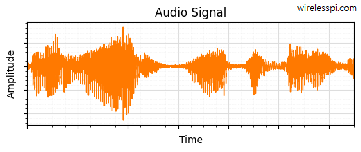
To investigate the answer, we start with an example audio signal drawn in the figure below that displays amplitude versus time for some spoken words.
For a comparison, a radio signal with digital modulation is plotted below.
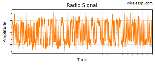
Clearly, both audio and radio signals are simple real waveforms plotted with time. Why then I/Q processing is not common in traditional audio applications but an integral part of radio communications? For this purpose,
- Part 1 delves into the significance of I/Q processing in wireless systems, and
- Part 2 broadens the scope, linking the I/Q signals (also known as quadrature signals) to Fourier Transform, the most important tool in all signal processing applications.
Let us start with the nature of an electromagnetic wave.
An Electromagnetic Messenger
Wireless systems employ an electromagnetic wave acting as a carrier of information hidden in the variations of its parameters.
The Sinusoidal Wave
This electromagnetic wave is produced by an oscillator through acceleration and deceleration of charges in the forward and reverse directions. Since the charges primarily oscillate back and forth, the wave exhibits a sinusoidal form.
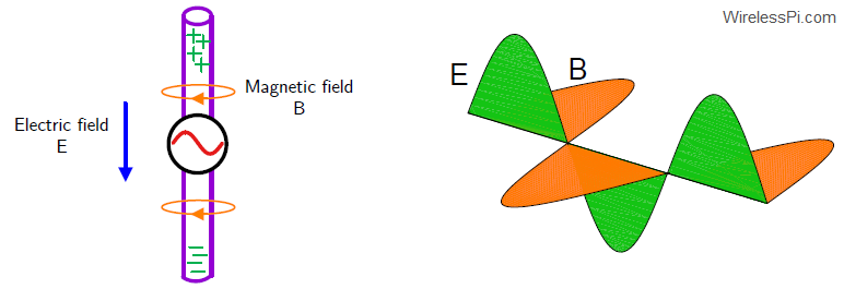
A reverse process occurs on the receive side. The impinging EM wave influences the electrons in the antenna through its electric and magnetic fields. The acceleration and deceleration of these electrons under the influence of these fields creates a tiny sinusoidal electrical signal.
In signal processing, a pure sinusoidal signal is also known as a tone. The title of this article refers to this tone, as we will now see how this simple signal alone leads us towards a deep understanding of I/Q signals now and Fourier Transform later.
The Message
This sinusoidal wave can be written as
\[
x(t) = A \cos (\omega t + \phi)
\]
where
- $A$ is the amplitude,
- $\omega$ is the angular frequency, and
- $\phi$ is the phase shift.
I/Q Signals: Mystery # 1
Much of the confusion behind I/Q signals is hidden underneath the idea of phase. Therefore, instead of simply using the term phase, I will differentiate between the following expressions.
- Phase shift: This occurs when the waveform is displaced to the right or left from the zero time reference (not aligned with how the waveform is defined, e.g., with peak of a cosine or zero of a sine).
- Phase angle: This is the angle of a complex number in the plane formed by real and imaginary parts (more on this later). A good example of phase angle is the carrier phase offset between the Tx and Rx local oscillators.
Are these different versions of phase related to each other? The answer depends on the context and I will use the term phase shift or phase angle in the article for clarity.
Any of the above three parameters of a sinusoid can be altered with time to encode a message. The information in this message can be
- user-generated (e.g., wireless communications),
- arising from the laws of nature (e.g., radar, astronomy, remote sensing, biomedical), or
- both (e.g., navigation and positioning systems, beamforming).
To people familiar with signal processing, the logical route from here is to show that the phase shift of the sinusoid can only be measured in two dimensions, not one. But this approach will require the reader to understand orthogonality, which is where we go next.
Are There More Carriers?
In bygone times, messages were delivered either by homing pigeons traveling long distances or by spies arriving on horseback at the gates of a walled city. For obvious reasons, having more messengers was essential for surveillance and governance. Therefore, kingdoms used to rely on flocks of pigeons and networks of spies.

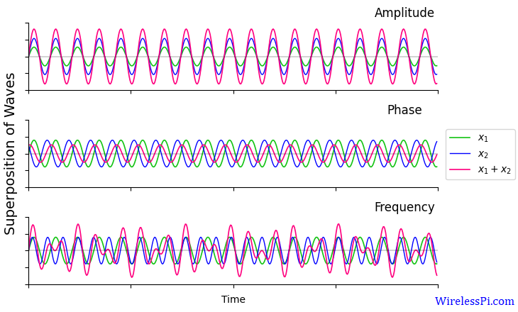
Similarly, the question is how to get more carriers in the case of a sinusoidal wave to deliver more messages. To achieve this goal, there should be no interference among the carriers as a fundamental requirement. However, as shown in the figure below, when two carriers with different amplitudes (or phase shifts or frequencies) combine, they create a wave with an amplitude (or phase shift or frequency) that differs from both of the original carriers. Clearly, two waves cannot coexist without meddling with each other.
To solve this problem, we need to learn about orthogonality.
A Numerical Prism
In mathematics, orthogonality is a concept that generalizes the geometric idea of perpendicularity to linear algebra.
Orthogonality
To understand why orthogonality is important, consider a common example of our 3D space where the vectors x, y and z are at $90^\circ$ to each other.
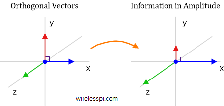
Any point in this 3D space can be written as a combination of the basis vectors with x, y and z coordinates.
\[
\mathbf{r} = x \mathbf{i} + y\mathbf{j}+ z\mathbf{k}
\]
where $\mathbf{i}$, $\mathbf{j}$ and $\mathbf{k}$ are the unit vectors in those dimensions. No matter how far we travel in x-direction, there is absolutely no change in y and z coordinates. This is orthogonality.
As shown in the figure depicting the superposition of waves before, even smooth sinusoids are not orthogonal to each other since their superposition is not zero. However, if these sinusoids are passed through an algorithm implementing some arithmetic operation, we have a chance to achieve orthogonality at the output. This is illustrated in the figure below.
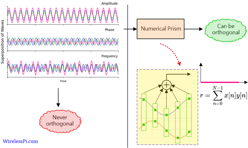
Let us call this algorithm a numerical prism. Next, we see how a simple operation can indeed act as such a prism.
The Dot Product
In a world of machine learning and artificial intelligence, extracting an ever increasing amount of information from the same waveform has become possible. Nevertheless, since signal processing engineers cannot spend millions of dollars, they rely on simple mathematical operations for efficient implementation of algorithms.
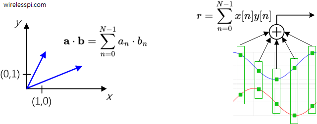
What we are seeking here is a simple technique that gives us more sinusoidal carriers of information unaffected by one another. Let us take help from the vectors themselves. When do two vectors not interfere with each other? When the angle between them is $90^\circ$ or the cosine of the angle is zero.
\[
\mathbf{a}\cdot \mathbf{b} = |\mathbf{a}|\cdot |\mathbf{b}|\cdot \cos \theta = 0, \quad \text{or}\quad \theta = 90^\circ
\]
From a geometrical viewpoint, when the dot product between the vectors is zero.
Just in case you are wondering where the cosine came from: In a 2D space, and without any loss of generalization, assume that one of the two vectors is $(1,0)$. In this case, the dot product is simply the projection or x-coordinate of the other vector, which brings the cosine of the angle between them into the expression.
From an algebraic viewpoint (which can be shown to be equivalent to geometric interpretation using the law of cosines), the dot product of two length-$N$ vectors is defined as the sum of their element-by-element products.
\[
\begin{align*}
r &= \mathbf{a}\cdot\mathbf{b} = \sum_{n=0}^{N-1}a_n b_n \\\\
&= a_0b_0+ a_1b_1 + \cdots + a_{N-1}b_{N-1}
\end{align*}
\]
Vectors $\mathbf{a}=[1,0]$ and $\mathbf{b}=[0,1]$ represent a common example of unit vectors in 2D space. But the same idea can be extended to other pairs like $\mathbf{a}=[2,3]$ and $\mathbf{b}=[6,-4]$ where we have
\[
r = \mathbf{a}\cdot\mathbf{b} = 2(6) + 3(-4) = 0
\]
In the domain of signals, this dot product is similar to correlation at zero lag defined by
\[
\begin{align*}
r &= \sum_{n=0}^{N-1} x[n]\cdot y[n]\\\\
&= x[0]y[0]+ x[1]y[1] + \cdots + x[N-1]y[N-1]
\end{align*}
\]
This process is illustrated in the figure below.
In continuous time, the summation becomes an integration and can be written as
\[
r = \int_{\tau_1}^{\tau_2} x(t)y(t)dt
\]
where the integral is taken over a defined interval.
Since a sinusoid has only three parameters, namely amplitude, phase shift and frequency, we now explore which of them can facilitate orthogonality.
Orthogonality in Amplitude
Let us start with two sinusoids stored in digital memory with different amplitudes but same frequency and phase shift. Then, we can write
\[
\begin{align*}
r = \int A_1\cos (\omega t + \phi)\cdot A_2 \cos (\omega t + \phi)dt &= A_1A_2\int \cos^2 (\omega t + \phi)dt \\\\
&\neq 0
\end{align*}
\]
In words, the reasoning is as follows.
- When the dot product or correlation of these two signals is computed, the amplitude can clearly be taken out as common.
- The result is a dot product of cosine with itself.
- Since a number multiplied with itself is its square, this sum of squares is a large number without any cancellation of positive values with negative ones during the integration process.
- As a consequence, it can never be zero.
We conclude that orthogonality in amplitude is not possible with a prism that computes a summation of element-wise products. Anyone who develops a different numerical prism that ensures orthogonality in amplitude is going to be famous.
Orthogonality in Phase Shift
Remember that only amplitudes exist in a real world, e.g., in a computer memory, as shown in the figure below.
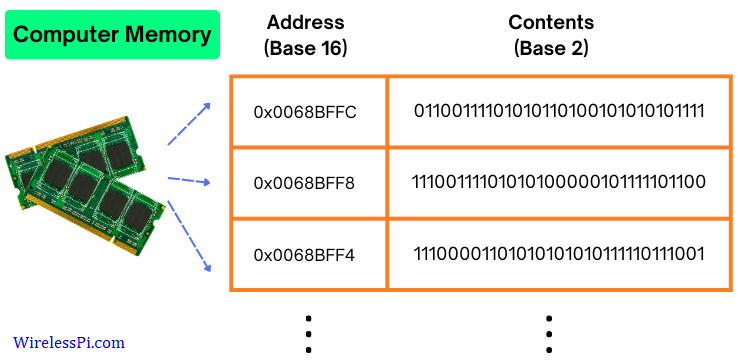
Can you see any phase or frequency in the signal values stored in the memory above? No, we define these parameters ourselves! This insight gives a hint that it might be possible to have a signal with different phase shifts whose dot product is equal to zero.
Phase Shifted Sinusoids
To test this idea, the figure below plots a cosine with its shifted versions. When a correlation or dot product is computed between $\cos (\omega t)$ and $\cos (\omega t + \theta)$, the output is nonzero for all values except when the phase shift is $\pm 90^\circ$.
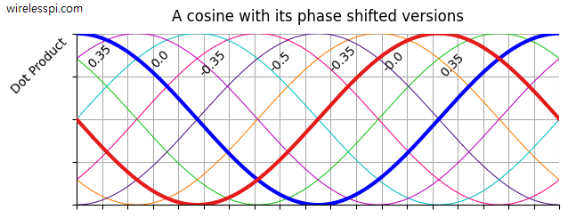
In other words, the sum of element-wise products of a cosine (shown in blue in the figure above) is zero for two versions: a negative sine (red) and a sine (cyan). This can also be verified from the following relation.
\[
\cos\left(\omega t \pm 90^\circ\right) = \cos (\omega t) \cos 90^\circ \mp \sin (\omega t) \sin 90^\circ = \mp \sin(\omega t)
\]
Since these two waves $\mp \sin(\omega t)$ are the same except for an amplitude scaling of $-1$, we can only retain one as orthogonal to cosine. Staying with the positive phase shift ($+90^\circ$) in cosine above, we choose the negative sine wave as the orthogonal signal.
Mathematically, we can verify this orthogonality as (including an immaterial factor of $2$)
\[
r = 2\int_{\tau_1}^{\tau_2} \cos (\omega t)\cdot \sin (\omega t) = \int_{\tau_1}^{\tau_2} \sin (2\omega t) = 0
\]
The result is zero under all conditions.
- If the integral is taken over an integer number of periods, the area under the curve $\sin (2\omega t)$ contains an equal number of positive and negative halves. They cancel each other out.
- When $\tau_1=-\tau_2$, any part of the signal from $0$ to $-\tau_2$ is exactly the same but with opposite sign as the part from $0$ to $\tau_2$. This is because $\sin (2\omega t)$ is an odd signal. Hence, their sum is zero.
- Even for an interval spanning a non-integer number of periods, this relation is approximately zero for large $\omega$. Why? Because a high frequency or diminishing time period implies that very little area would remain outside the balanced positive and negative halves.
This can be seen as follows.
\[
\begin{align*}
r = \int_{\tau_1}^{\tau_2} \sin (2\omega t) &= \frac{-\cos (2\omega t)}{2\omega}\Bigg|_{\tau_1}^{\tau_2} = \frac{\cos (2\omega \tau_1)\, – \cos (2\omega \tau_2)}{2\omega}\\\\
&= \frac{\sin[\omega(\tau_2+\tau_1)]\sin[\omega(\tau_2-\tau_1)]}{\omega} \le \frac{1}{\omega} \approx 0
\end{align*}
\]The second last step follows from $|\sin(\omega t)| \le 1$. Hence, the above expression goes to zero for a sufficiently high frequency in the denominator. Indeed, carrier frequencies are high in wireless communications.
This orthogonality in phase shift implies that we have two carriers, not one! In addition to the original sinusoidal wave (a cosine), we have another sinusoidal wave (negative sine) to carry information as a messenger, as long as we implement some version of dot product at the receiver.

Mathematically, we write
\[
\begin{aligned}
\text{1st carrier} \quad &\rightarrow \quad \cos \omega t\\
\text{2nd carrier} \quad &\rightarrow \quad -\sin \omega t
\end{aligned}
\]
Next, we explore how these two carriers can be used in a communication system as an example. Later, we expand the idea into general complex signal processing.
A Communication System Example
The two possible options to modulate these phase orthogonal sinusoids are amplitude and frequency. Being spectrally efficient, it is the amplitude modulation that is more widely used. One example of this concept is Quadrature Amplitude Modulation (QAM), the most widely used modulation scheme in modern communication systems.
I/Q Modulation
We can vary the amplitude of the these two waves, say $I_m$ on cosine and $Q_m$ on negative sine, independent of each other (an explanation of this notation follows shortly), where $m$ is the time index for units of information ($m=0,1,2,\cdots$).
Benefiting from orthogonality, we can then combine these two streams into a single waveform before sending them into the physical medium (wireless channel, coaxial cable, etc.) at the carrier frequency $\omega$. The transmitted signal can then be written as
\begin{equation}\label{equation-iq}
x(t) = I_m \cos (\omega t) \,- Q_m \sin (\omega t)
\end{equation}
This can be seen in the block diagram below where the time index $m$ is not shown for clarity. At the Tx side, the $I$ and $Q$ amplitude streams can be seen as two parallel wires before they are mixed with respective sinusoids and summed together to form a single signal $x(t)$ of Eq (\ref{equation-iq}) that is sent into the air.
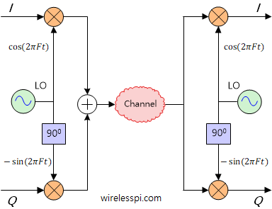
All this implies that an I/Q signal is a sum of an amplitude times a zero-phase cosine wave and another amplitude times a zero-phase (negative) sine wave.
Next, we investigate how to choose these $I$ and $Q$ values.
$I$ and $Q$ at the Tx
At the Tx side in 4-QAM, for instance, the 4 modulation symbols are shown on the left side of the figure below.
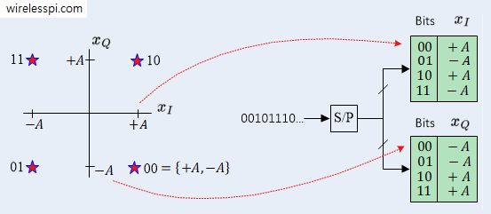
Assume that the bit sequence 00101110 needs to be transmitted. There are $4=2^2$ distinct symbols which can be addressed with a pair of bits.
- In the above figure, the first two bits 00 are mapped to $\{+A,-A\}$.
- Looking at the output of the $I_m$ and $Q_m$ lookup tables for address 00, we have
\[
00 \quad \rightarrow \quad \{+A,-A\} \qquad \rightarrow \qquad I_m = +A, \quad Q_m = -A
\] - Using Eq (\ref{equation-iq}), these two amplitudes are mixed with cosine and negative sine, respectively, to form the eventual waveform as
\begin{equation}\label{equation-qam-example}
x(t) = +A \cos (\omega t) \,- (-A)\sin(\omega t)
\end{equation}
which is the waveform sent into the medium.
We now explore how these $I$ and $Q$ values are extracted at the other side.
$I$ and $Q$ at the Rx
At the Rx side during downconversion, this single incoming signal is mixed with respective sinusoids to remove the carriers and extract $I$ and $Q$ amplitude streams. This is possible due to the orthogonality of these sinusoids and can be verified using trigonometric identities as follows.
- Multiply $x(t)$ of Eq (\ref{equation-iq}) with a perfectly synchronized cosine with compensated phase offset and frequency offset (including the scaling factor of $2$). Using $2\cos^2\theta$ $=$ $1+\cos2\theta$,
\[
\begin{align*}
x(t) \cdot 2\cos (\omega t) &= \left[I_m \cos (\omega t) \,- Q_m \sin (\omega t)\right]\cdot 2\cos (\omega t)\\\\
&= I_m +\underbrace{I_m \cos (2\omega t)-Q_m \sin (2\omega t)}_{\text{lowpass filtered}}\\
&\approx I_m
\end{align*}
\]where the double frequency terms are eliminated by a lowpass filter.
- Multiply $x(t)$ of Eq (\ref{equation-iq}) with negative sine (including the scaling factor of $2$). Using $2\sin^2\theta$ $=$ $1-\cos2\theta$,
\[
\begin{align*}
-x(t) \cdot 2\sin (\omega t) &= -\left[I_m \cos (\omega t) \,- Q_m \sin (\omega t)\right]\cdot 2\sin (\omega t)\\\\
&= Q_m\,- \underbrace{I_m \sin (2\omega t)-Q_m \cos (2\omega t)}_{\text{lowpass filtered}}\\
&\approx Q_m
\end{align*}
\]
These $I$ and $Q$ streams can be seen coming out as two parallel wires on the Rx side of the above block diagram! As a consequence, the spectral efficiency of the channel increases by a factor of 2.
Something important to note: there are no complex numbers here yet! Before we explore the role of complex numbers, we need to investigate where the terms $I$ and $Q$ come from.
What are $I$ and $Q$ Signals?
The phase shifts of these two orthogonal waves need a reference with sine and cosine being the two options.
- In-phase: A cosine wave is chosen as the reference or in-phase part, from which the notation $I$ is extracted. Depending on the context, the term $I$ is used for any of the following three signals:
- the cosine wave: $\cos (\omega t)$
- the amplitude-modulated cosine wave: $I_m \cos (\omega t)$
- the amplitude riding over this cosine: $I_m$ (the most common usage in signal processing)
- Quadrature: In astronomy, the term quadrature refers to the position of a planet when it is $90^\circ$ from the sun as viewed from the earth. Since a negative sine wave has a phase difference of $90^\circ$ with the reference cosine wave, it is known as the quadrature part from which the notation $Q$ is extracted. Again, the $Q$ term is used for any of the following three signals:
- the negative sine wave: $-\sin (\omega t)$
- the amplitude-modulated negative sine wave: $-Q_m \sin (\omega t)$
- the amplitude riding over this negative sine: $Q_m$ (the most common usage in signal processing)
This brings up the question of how to treat these two amplitudes, as a 2D vector or a single complex number.
Where Does the Complex Plane Come from?
As shown in the figure below, carrier generation and multiplication by $I$ and $Q$ streams in the frontend is a 1D signal processing operation in each arm. However, to prepare these streams for transmission on one side and demodulation of data bits at the other side, these two signals, $I$ and $Q$, need to be treated as a 2D number within the digital processing machine.
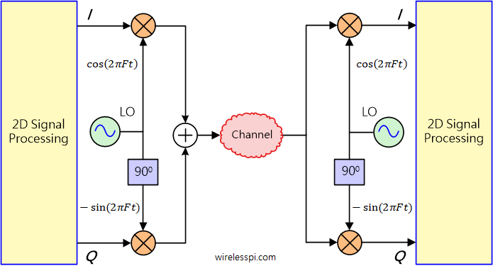
This gives rise to the following two possibilities:
- a 2D plane of vectors with matrix operations, or
- a complex plane.
While complex numbers do have some similarities with vectors in a 2D plane, they are not identical.
2D Vectors vs Complex Numbers
In the 2D geometric plane, points are represented as pairs of real numbers $(x, y)$, while in the complex plane, points are represented as a single complex number $x + jy.$ Some of its implications are the following.
- Addition: Adding two 2D vectors $(x_1,y_1)$ and $(x_2,y_2)$ results in $(x_1+x_2,y_1+y_2)$, which is similar to how adding two complex numbers $x_1+jy_1$ and $x_2+jy_2$ leads to $(x_1+x_2) + j(y_1+y_2)$. Same is the case for subtraction.
- Multiplication: Multiplication is defined in complex numbers just like real numbers. For example, multiplying $x_1+jy_1$ and $x_2+jy_2$ gives the following result.
\[
(x_1+jy_1)(x_2+jy_2) = (x_1x_2-y_1y_2) + j(x_1y_2+y_1x_2)
\]In a vector world of dot products, cross products, element-wise products and so on, multiplication is not as straightforward an operation. However, consider forming a 2D matrix from any complex number as follows.
\[
x_1+jy_1 \rightarrow \begin{bmatrix}x_1 & -y_1 \\ y_1 & x_1 \end{bmatrix}
\]Then, the multiplication of two 2D matrices yields
\[
\begin{bmatrix}x_1 & -y_1 \\ y_1 & x_1 \end{bmatrix}\begin{bmatrix}x_2 & -y_2 \\ y_2 & x_2 \end{bmatrix} = \begin{bmatrix}x_1x_2-y_1y_2 & -(x_1y_2+y_1x_2) \\ x_1y_2+y_1x_2 & x_1x_2-y_1y_2 \end{bmatrix}
\]Compare the first column above with the multiplication result of complex numbers. Although both give the same answer, complex numbers handle this product just like real numbers while vector processing has to go through a complicated route.
- Division: Even more problems emerge with division. In real numbers, when $x_1$ is divided by $x_2$, we can write
\begin{equation}\label{equation-iq-signals-real-division}
\frac{x_1}{x_2} = z \qquad \text{or}\qquad x_1 = zx_2 = x_2z
\end{equation}For complex numbers, we can cancel the imaginary number $j$ in the denominator using arithmetic rules to find the result.
\[
\frac{x_1+jy_1}{x_2+jy_2} = \frac{x_1+jy_1}{x_2+jy_2}\cdot \frac{x_2-jy_2}{x_2-jy_2} = \frac{x_1x_2+y_1y_2+j(y_1x_2-y_2x_1)}{x_2^2+y_2^2}
\]Matrix division, however, leads to two problems.
- If the matrix $\mathbf{X_2}$ is invertible, matrix multiplication is not commutative. Analogous to division in real numbers in Eq (\ref{equation-iq-signals-real-division}), we have
\[
\mathbf{X_1X_2^{-1}} = \mathbf{Z} \qquad \text{or} \qquad \mathbf{X_1} = \mathbf{ZX_2} \neq \mathbf{X_2Z}
\]i.e., these are two distinct matrices.
- If the matrix $\mathbf{X_2}$ is not invertible (i.e., its determinant is 0 or it is a non-square matrix), then solutions to the above expressions either will not exist or will not be unique.
Therefore, the concept of matrix division is not easily justified.
- If the matrix $\mathbf{X_2}$ is invertible, matrix multiplication is not commutative. Analogous to division in real numbers in Eq (\ref{equation-iq-signals-real-division}), we have
From the above description alone, complex numbers already appear to be more suitable for 2D signal processing operations. But Euler’s formula practically sealed the deal.
Euler’s Formula
In 1748, Leonhard Euler derived a formula that combined the real and imaginary parts of a complex number into a single expression.
\[
e^{j\theta} = \cos\theta+j\sin\theta
\]
This enables us to express any complex number from rectangular coordinates to polar coordinates as a single compact number.
\[
z = x+ jy = |z|e^{j\theta}
\]
where $|z|$ is the magnitude and $\theta$ is the phase angle of $z$.
\begin{equation}\label{equation-phase-definition}
|z| = \sqrt{x^2+y^2}, \qquad \text{and}\qquad \theta = \tan^{-1}\frac{y}{x}
\end{equation}
Most people derive this result by power series expansions of the exponential and cosine/sine expressions but I find its lack of intuitiveness unappealing. To keep this article brief, I am providing references for an interested reader who wants to understand these topics in a better way.
- What is the origin of complex numbers and signals?
- Why does the constant $e$ appear in the representation of complex numbers (I highly recommend this one where I demonstrate how like a machine press, $e$ compresses an infinite number of rotations – disguised as multiplications – into a single quantity).
- What is the intuitive reasoning behind multiplication and division of complex numbers?
This brings us to the following conclusion.
Why Complex Numbers?
As opposed to the common belief, there is no inherent requirement for communication systems to adhere to complex signal processing! Electrical engineers prefer complex values for many reasons, the chief among them being that complex numbers, owing to rectangular and more compact polar representation, adhere to all the usual rules of algebra, particularly multiplication and division, just like real numbers. This helps tremendously in the reduction of trigonometric expressions into simple exponential form.
An example of this complex signal processing is a Phase Locked Loop (PLL) at the Rx side which estimates the incoming carrier phase and compensates for its rotation using complex operations.
In summary, the complex plane provides a powerful and elegant way to represent, analyze, and manipulate signals in signal processing. It offers mathematical tools and insights that are not easily accessible in the 2D real plane, making it the preferred choice for many signal processing applications.
A Time Domain I/Q Signal
In light of the above discussion, a single sample of an I/Q signal can be constructed as follows.
Generating an I/Q Sample in a Laboratory
Every sample of an I/Q signal has a magnitude and a phase. This phase angle, defined in Eq (\ref{equation-phase-definition}), is reproduced below.
\[
\theta = \tan^{-1}\frac{Q}{I}
\]
The phase angle is the orientation of the complex number on the $IQ$ plane.
To explain this idea, let us build a 5V DC signal with $60^\circ$ of phase in the laboratory with two power supplies. We can write
\[
\begin{aligned}
I \quad \rightarrow \quad 5\cos 60^\circ &= 2.5 \\
Q \quad \rightarrow \quad 5\sin 60^\circ &= 4.3
\end{aligned}
\]
This complex DC signal is shown as a red square on an oscilloscope in the figure below.
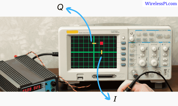
Recall that a complex number is simply two real numbers in parallel while $j$ exists in our own heads only. Therefore, it is important to understand that the above plot is $Q$ with respect to $I$, not time.
What happens when this complex number starts rotating with time? This is a question explored in Part 2.
An I/Q Signal
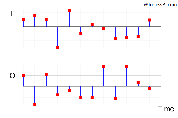
At the most elementary level, a digital I/Q signal can be described as follows.
- A digital signal is nothing but a sequence of numbers.
- A complex number is made up of two components: a real part and an imaginary part.
- A digital I/Q signal is simply two real signals in parallel, treated as a sequence of complex numbers!
In a digital machine, this complex sequence is actually composed of two real sequences evolving with time in which one represents the real arm and the other the imaginary arm as drawn below.
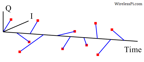
The same example in a 3D plane consisting of $I$ and $Q$ against time is drawn in the figure below. Compare these $I$ and $Q$ values (or simply their signs) with their counterparts in the above figure.
The next figure plots the first four samples in an I/Q plane for clarity. Compare them with the first four samples in the above 3D sequence.
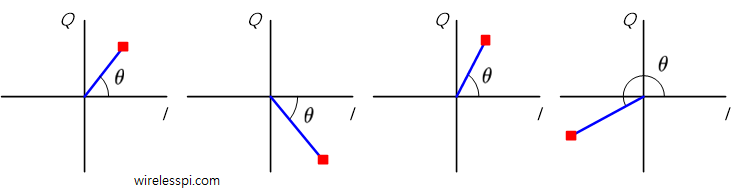
As a consequence, we could have easily called the I/Q signal a complex signal (with an understanding that the complex convention is in our heads)! Observe how each I/Q sample in a complex plane has a magnitude and a phase angle.
Conclusion
An I/Q signal is nothing but two real signals in parallel which can be treated as simply a sequence of complex numbers. In such a framework, the length represents the magnitude while the orientation of a complex number for each sample represents the phase angle, on which rules of complex arithmetic can be applied. There is more to this story connecting these ideas that is described in Part 2 on Fourier Transform.
At this stage, a signal processing beginner can go on to read Part 2. However, an advanced reader can explore below the contradiction in phase modulation related to I/Q signals.
Appendix: I/Q and Phase Modulation
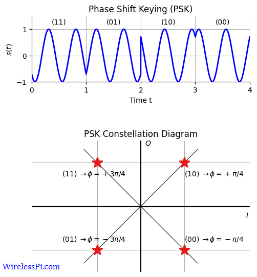
Phase Shift Keying (PSK) is a digital modulation scheme in which the phase of a sinusoid is shifted according to the data bits to convey the message. For example, in QPSK, the four bit pairs 00, 01, 10 and 11 can represent four phase shifts of a sinusoid.
\[
\begin{align*}
00 &\quad \rightarrow \quad \phi = -\frac{\pi}{4}\\
01 &\quad \rightarrow \quad \phi = -\frac{3\pi}{4}\\
10 &\quad \rightarrow \quad \phi = +\frac{\pi}{4}\\
11 &\quad \rightarrow \quad \phi = +\frac{3\pi}{4}\\
\end{align*}
\]
The resulting constellation diagram and the modulated waveform are drawn in the figure below.
Then the PSK waveform can be written as
\begin{equation}\label{equation-psk}
x(t) = A \cos (\omega t + \phi_m)
\end{equation}
where the phase $\phi_m$ depends on the data bits chosen at time $m=0,1,2,\cdots$. This brings us to a surprising contradiction.
Contradiction
We already exhausted the phase part to distinguish the two carriers, $\cos (\omega t)$ and $-\sin(\omega t)$, to achieve orthogonality. Then, how can the phase shift of the above sinusoid be modulated with information bits in the above I/Q diagram? Will this not give rise to interference?
This contradiction can be resolved as follows. Consider the trigonometric identity $\cos (\alpha+\beta)$ $=$ $\cos \alpha \cos \beta$ $-$ $\sin\alpha \sin\beta$ to open the PSK expression in Eq (\ref{equation-psk}).
\begin{equation}\label{equation-identity}
x(t) = A \cos\phi_m \cdot\cos(\omega t) \,- A\sin\phi_m\cdot \sin(\omega t)
\end{equation}
This can become the same expression as that for 4-QAM in Eq (\ref{equation-iq})
\[
x(t) = I_m\cos(\omega t)\,-Q_m\sin(\omega t)
\]
if
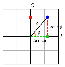
\begin{equation}\label{equation-inphase-quadrature}
I_m = A\cos \phi_m \qquad \text{and} \qquad Q_m = A \sin \phi_m,
\end{equation}
Using $\cos^2\phi_m+\sin^2\phi_m=1$ and $\tan\phi_m=\sin\phi_m/\cos\phi_m$, respectively, both $A$ and $\phi$ can easily be determined.
\begin{equation}\label{equation-amplitude-phase}
A = \sqrt{I_m^2+Q_m^2} \qquad \text{and}\qquad \phi_m = \tan^{-1}\frac{Q_m}{I_m}
\end{equation}
An I/Q plane illustrating such a connection is drawn in the figure below.
Plugging them back in Eq (\ref{equation-psk}) results in
\begin{equation}\label{equation-iq-signals}
x(t) = A \cos (\omega t+\phi_m) = \sqrt{I_m^2+Q_m^2} \cos \left(\omega t \,+ \tan^{-1}\frac{Q_m}{I_m} \right)
\end{equation}
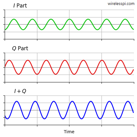
In words, the combined signal from modulated cosine and negative sine also becomes a third sinusoid with a distinct amplitude and phase shift! This is drawn in the figure below (for a given $m$) where both amplitude and phase shift of the sum $I+Q$ can be observed as different from either of the constituent $I$ and $Q$ signals.
I/Q Signals: Mystery # 2
This is unlike vectors where x and y axes are still visible while drawing a resultant vector. Imagine how strange it would seem if the following relation was true.
\[
2.5x + 4.3y = -3.7x
\]
On the other hand, when two phase-orthogonal sinusoids are modulated in amplitude and summed together, they effectively disappear in the resultant third sinusoid. This is another reason behind the puzzle of I/Q signals.
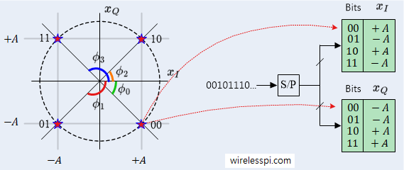
Keep in mind that this phase modulation is primarily intended for understanding and analysis purposes, rather than practical implementation. Nearly all actual modems implement PSK through amplitude processing of complex numbers, just like a QAM signal. This becomes possible by observing the figure below where 4 modulation phases in QPSK can easily be replaced by a lookup table with corresponding $I$ and $Q$ amplitudes described before in 4-QAM.
To summarize, we process two amplitudes of an I/Q signal in a digital machine and combine them to send into the air a single sinusoid modulated in phase. In the Rx after downconversion, it is only the underlying $I$ and $Q$ amplitudes again that are processed for demodulation.