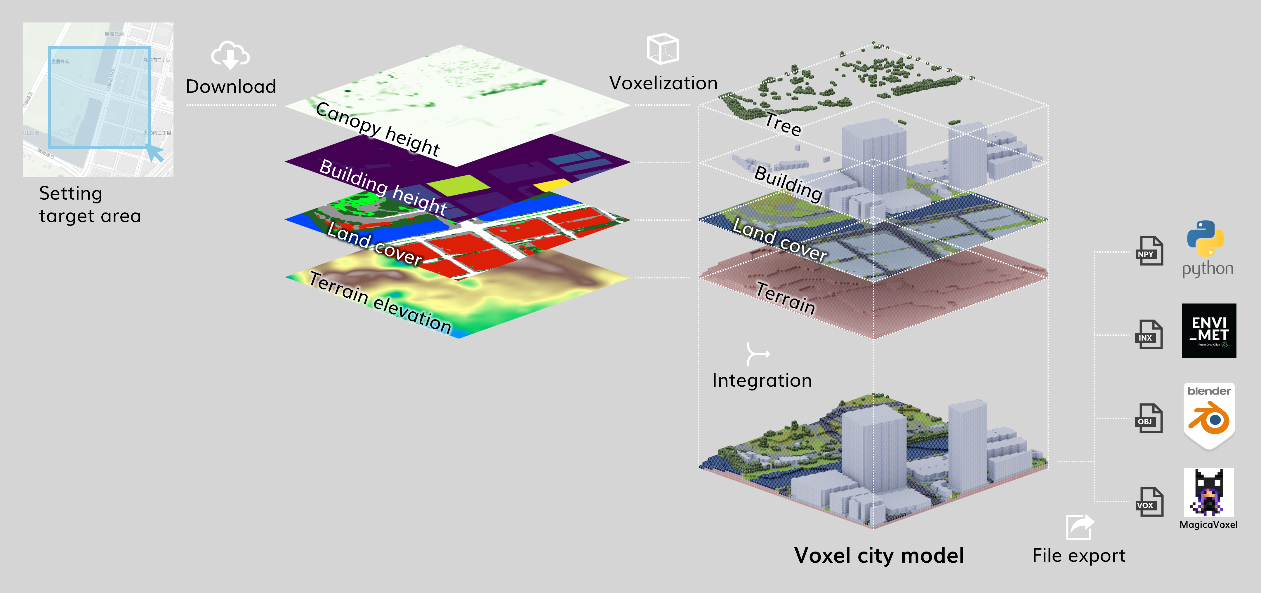
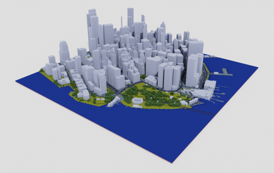
voxcity is a Python package that provides a seamless solution for grid-based 3D city model generation and urban simulation for cities worldwide. VoxCity's generator module automatically downloads building heights, tree canopy heights, land cover, and terrain elevation within a specified target area, and voxelizes buildings, trees, land cover, and terrain to generate an integrated voxel city model. The simulator module enables users to conduct environmental simulations, including solar radiation and view index analyses. Users can export the generated models using several file formats compatible with external software, such as ENVI-met (INX), Blender, and Rhino (OBJ). Try it out using the Google Colab Demo or your local environment. For detailed documentation, API reference, and tutorials, visit our Read the Docs page.
Integration of Multiple Data Sources:
Combines building footprints, land cover data, canopy height maps, and DEMs to generate a consistent 3D voxel representation of an urban scene.
Flexible Input Sources:
Supports various building and terrain data sources including:
Building Footprints: OpenStreetMap, Overture, EUBUCCO, Microsoft Building Footprints, Open Building 2.5D
Land Cover: UrbanWatch, OpenEarthMap Japan, ESA WorldCover, ESRI Land Cover, Dynamic World, OpenStreetMap
Canopy Height: High Resolution 1m Global Canopy Height Maps, ETH Global Sentinel-2 10m
Customizable Domain and Resolution:
Easily define a target area by drawing a rectangle on a map or specifying center coordinates and dimensions. Adjust the mesh size to meet resolution needs.
Integration with Earth Engine:
Leverages Google Earth Engine for large-scale geospatial data processing (authentication and project setup required).
Output Formats:
ENVI-MET: Export INX and EDB files suitable for ENVI-MET microclimate simulations.
MagicaVoxel: Export vox files for 3D editing and visualization in MagicaVoxel.
OBJ: Export wavefront OBJ for rendering and integration into other workflows.
Analytical Tools:
View Index Simulations: Compute sky view index (SVI) and green view index (GVI) from a specified viewpoint.
Landmark Visibility Maps: Assess the visibility of selected landmarks within the voxelized environment.
Make sure you have Python 3.12 installed. Install voxcity with:
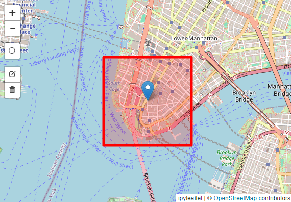
Use the GUI map interface to draw a rectangular domain of interest.
fromvoxcity.geoprocessor.drawimportdraw_rectangle_map_citynamecityname="tokyo"m, rectangle_vertices=draw_rectangle_map_cityname(cityname, zoom=15)
m
Option 3: Specify Center and Dimensions (for Jupyter Notebook)
Choose the width and height in meters and select the center point on the map.
fromvoxcity.geoprocessor.drawimportcenter_location_map_citynamewidth=500height=500m, rectangle_vertices=center_location_map_cityname(cityname, width, height, zoom=15)
m
Define data sources and mesh size (m):
building_source='OpenStreetMap'# Building footprint and height data sourceland_cover_source='OpenStreetMap'# Land cover classification data sourcecanopy_height_source='High Resolution 1m Global Canopy Height Maps'# Tree canopy height data sourcedem_source='DeltaDTM'# Digital elevation model data sourcemeshsize=5# Grid cell size in meterskwargs= {
"output_dir": "output", # Directory to save output files"dem_interpolation": True# Enable DEM interpolation
}
Generate voxel data grids and corresponding building geoJSON:
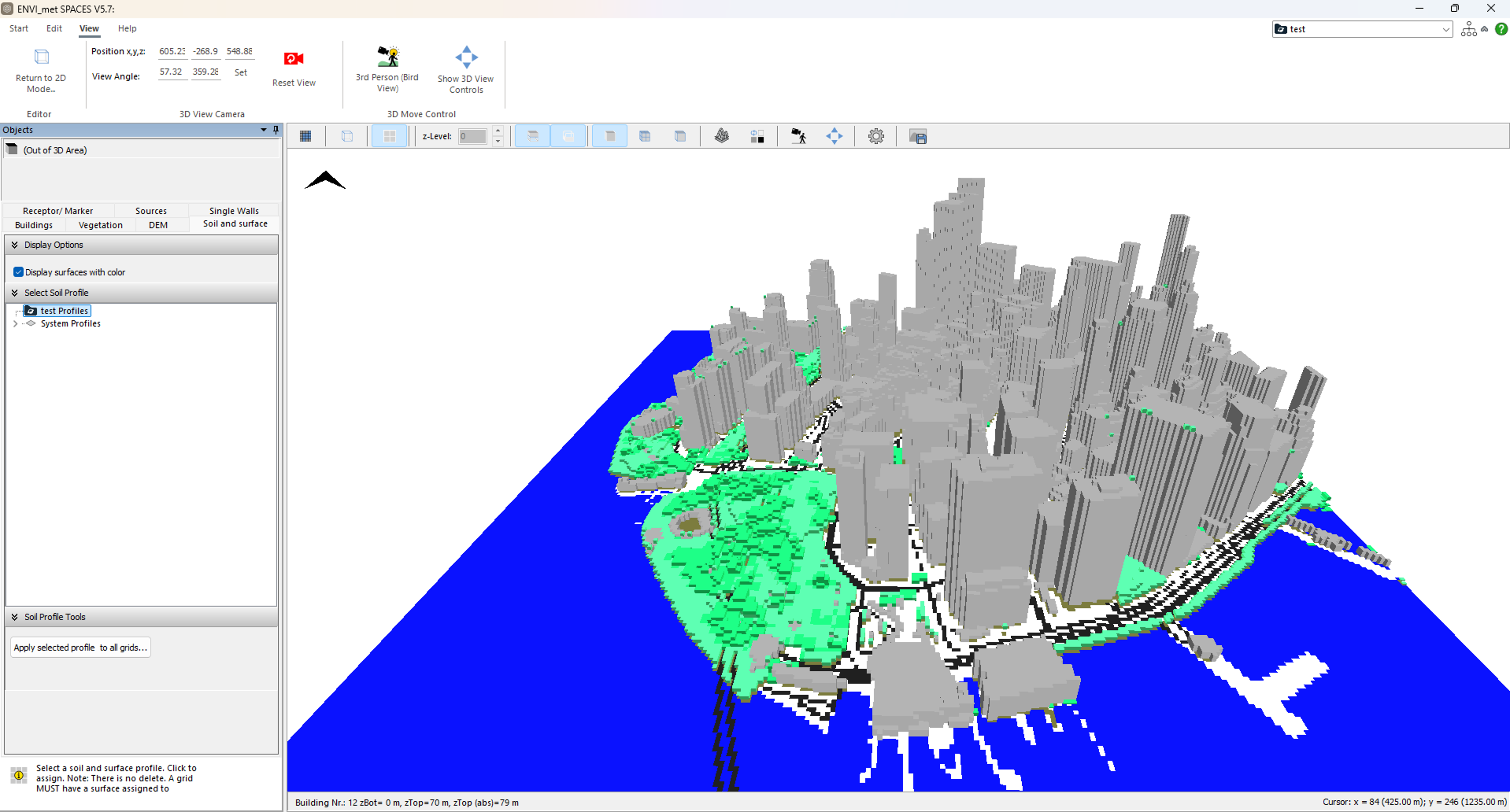
ENVI-MET is an advanced microclimate simulation software specialized in modeling urban environments. It simulates the interactions between buildings, vegetation, and various climate parameters like temperature, wind flow, humidity, and radiation. The software is used widely in urban planning, architecture, and environmental studies (Commercial, offers educational licenses).
fromvoxcity.exporter.envimetimportexport_inx, generate_edb_fileenvimet_kwargs= {
"output_directory": "output", # Directory where output files will be saved"author_name": "your name", # Name of the model author"model_description": "generated with voxcity", # Description text for the model"domain_building_max_height_ratio": 2, # Maximum ratio between domain height and tallest building height"useTelescoping_grid": True, # Enable telescoping grid for better computational efficiency"verticalStretch": 20, # Vertical grid stretching factor (%)"min_grids_Z": 20, # Minimum number of vertical grid cells"lad": 1.0# Leaf Area Density (m2/m3) for vegetation modeling
}
export_inx(building_height_grid, building_id_grid, canopy_height_grid, land_cover_grid, dem_grid, meshsize, land_cover_source, rectangle_vertices, **envimet_kwargs)
generate_edb_file(**envimet_kwargs)
Example Output Exported in INX and Inported in ENVI-met
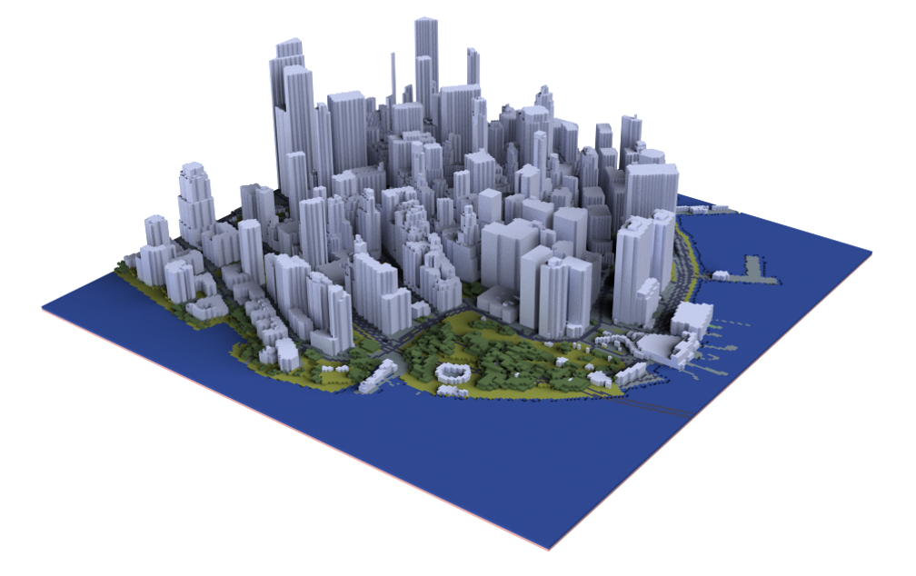
fromvoxcity.exporter.objimportexport_objoutput_directory="output"# Directory where output files will be savedoutput_file_name="voxcity"# Base name for the output OBJ fileexport_obj(voxcity_grid, output_directory, output_file_name, meshsize)
The generated OBJ files can be opened and rendered in the following 3D visualization software:
Twinmotion: Real-time visualization tool (Free for personal use)
Blender: Professional-grade 3D creation suite (Free)
Rhino: Professional 3D modeling software (Commercial, offers educational licenses)
Example Output Exported in OBJ and Rendered in Rhino
MagicaVoxel is a lightweight and user-friendly voxel art editor. It allows users to create, edit, and render voxel-based 3D models with an intuitive interface, making it perfect for modifying and visualizing voxelized city models. The software is free and available for Windows and Mac.
Example Output Exported in VOX and Rendered in MagicaVoxel
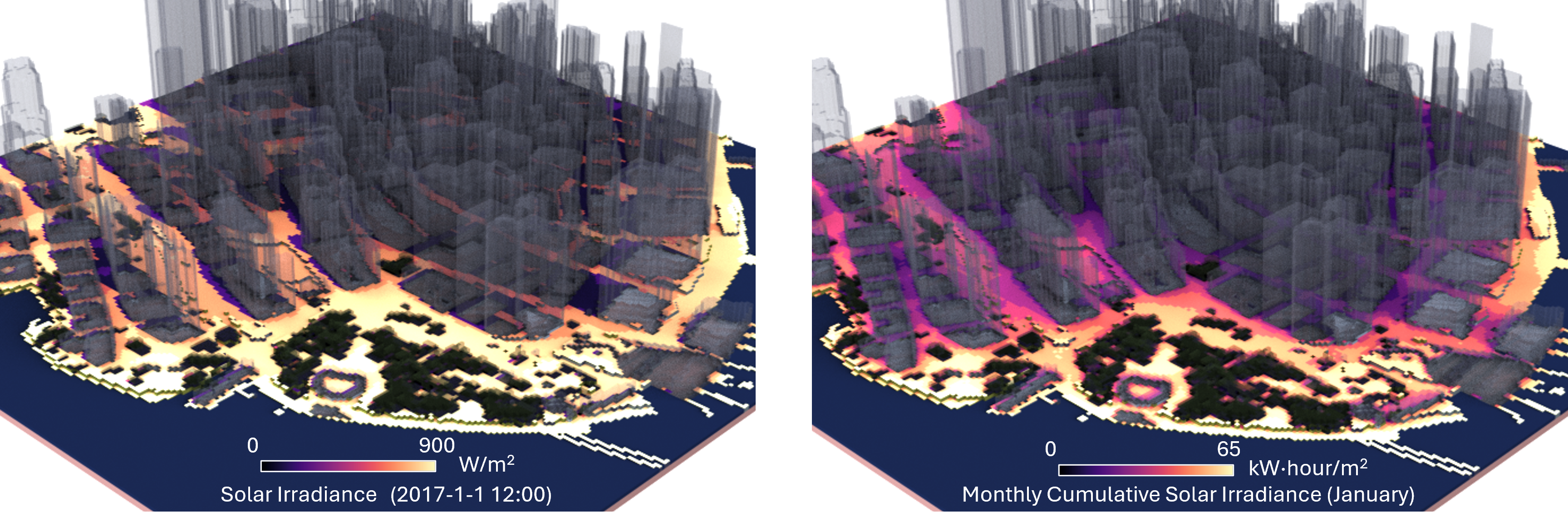
Compute Solar Irradiance:
fromvoxcity.simulator.solarimportget_global_solar_irradiance_using_epwsolar_kwargs= {
"download_nearest_epw": True, # Whether to automatically download nearest EPW weather file based on location from Climate.OneBuilding.Org"rectangle_vertices": rectangle_vertices, # Coordinates defining the area of interest for calculation# "epw_file_path": "./output/new.york-downtown.manhattan.heli_ny_usa_1.epw", # Path to EnergyPlus Weather (EPW) file containing climate data. Set if you already have an EPW file."calc_time": "01-01 12:00:00", # Time for instantaneous calculation in format "MM-DD HH:MM:SS""view_point_height": 1.5, # Height of view point in meters for calculating solar access. Default: 1.5 m"tree_k": 0.6, # Static extinction coefficient - controls how much sunlight is blocked by trees (higher = more blocking)"tree_lad": 1.0, # Leaf area density of trees - density of leaves/branches that affect shading (higher = denser foliage)"dem_grid": dem_grid, # Digital elevation model grid for terrain heights"colormap": 'magma', # Matplotlib colormap for visualization. Default: 'viridis'"obj_export": True, # Whether to export results as 3D OBJ file"output_directory": 'output/test', # Directory for saving output files"output_file_name": 'instantaneous_solar_irradiance', # Base filename for outputs (without extension)"alpha": 1.0, # Transparency of visualization (0.0-1.0)"vmin": 0, # Minimum value for colormap scaling in visualization# "vmax": 900, # Maximum value for colormap scaling in visualization
}
# Compute global solar irradiance map (direct + diffuse radiation)solar_grid=get_global_solar_irradiance_using_epw(
voxcity_grid, # 3D voxel grid representing the urban environmentmeshsize, # Size of each voxel in meterscalc_type='instantaneous', # Calculate instantaneous irradiance at specified timedirect_normal_irradiance_scaling=1.0, # Scaling factor for direct solar radiation (1.0 = no scaling)diffuse_irradiance_scaling=1.0, # Scaling factor for diffuse solar radiation (1.0 = no scaling)**solar_kwargs# Pass all the parameters defined above
)
# Adjust parameters for cumulative calculationsolar_kwargs["start_time"] ="01-01 01:00:00"# Start time for cumulative calculationsolar_kwargs["end_time"] ="01-31 23:00:00"# End time for cumulative calculationsolar_kwargs["output_file_name"] ='cummulative_solar_irradiance', # Base filename for outputs (without extension)# Calculate cumulative solar irradiance over the specified time periodcum_solar_grid=get_global_solar_irradiance_using_epw(
voxcity_grid, # 3D voxel grid representing the urban environmentmeshsize, # Size of each voxel in meterscalc_type='cumulative', # Calculate cumulative irradiance over time period instead of instantaneousdirect_normal_irradiance_scaling=1.0, # Scaling factor for direct solar radiation (1.0 = no scaling)diffuse_irradiance_scaling=1.0, # Scaling factor for diffuse solar radiation (1.0 = no scaling)**solar_kwargs# Pass all the parameters defined above
)
Example Results Saved as OBJ and Rendered in Rhino
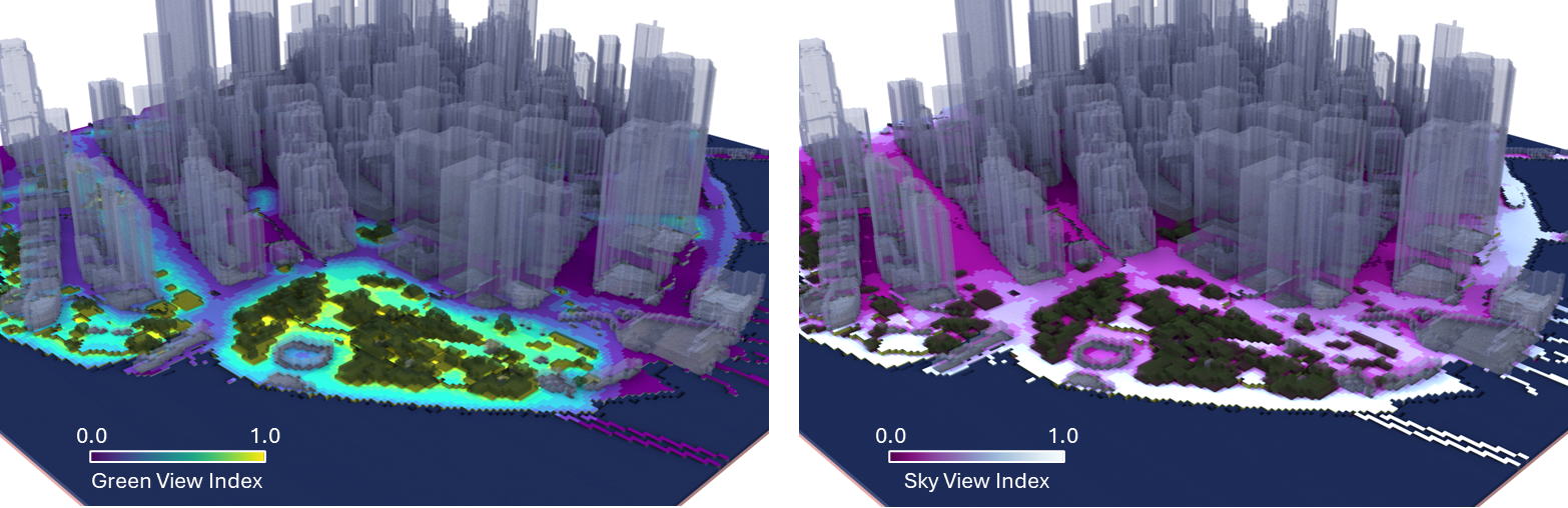
Compute Green View Index (GVI) and Sky View Index (SVI):
fromvoxcity.simulator.viewimportget_view_indexview_kwargs= {
"view_point_height": 1.5, # Height of observer viewpoint in meters"dem_grid": dem_grid, # Digital elevation model grid"colormap": "viridis", # Colormap for visualization"obj_export": True, # Whether to export as OBJ file"output_directory": "output", # Directory to save output files"output_file_name": "gvi"# Base filename for outputs
}
# Compute Green View Index using mode='green'gvi_grid=get_view_index(voxcity_grid, meshsize, mode='green', **view_kwargs)
# Adjust parameters for Sky View Indexview_kwargs["colormap"] ="BuPu_r"view_kwargs["output_file_name"] ="svi"view_kwargs["elevation_min_degrees"] =0# Start ray-tracing from the horizon# Compute Sky View Index using mode='sky'svi_grid=get_view_index(voxcity_grid, meshsize, mode='sky', **view_kwargs)
Example Results Saved as OBJ and Rendered in Rhino
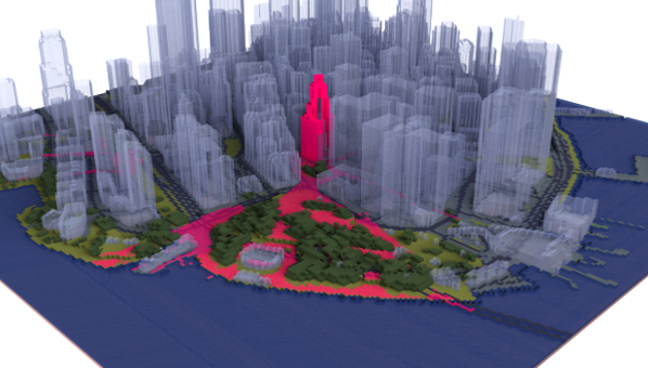
fromvoxcity.simulator.viewimportget_landmark_visibility_map# Dictionary of parameters for landmark visibility analysislandmark_kwargs= {
"view_point_height": 1.5, # Height of observer viewpoint in meters"rectangle_vertices": rectangle_vertices, # Vertices defining simulation domain boundary"dem_grid": dem_grid, # Digital elevation model grid"colormap": "cool", # Colormap for visualization"obj_export": True, # Whether to export as OBJ file"output_directory": "output", # Directory to save output files"output_file_name": "landmark_visibility"# Base filename for outputs
}
landmark_vis_map=get_landmark_visibility_map(voxcity_grid, building_id_grid, building_gdf, meshsize, **landmark_kwargs)
Example Result Saved as OBJ and Rendered in Rhino
fromvoxcity.geoprocessor.networkimportget_network_valuesnetwork_kwargs= {
"network_type": "walk", # Type of network to download from OSM (walk, drive, all, etc.)"colormap": "magma", # Matplotlib colormap for visualization"vis_graph": True, # Whether to display the network visualization"vmin": 0.0, # Minimum value for color scaling"vmax": 600000, # Maximum value for color scaling"edge_width": 2, # Width of network edges in visualization"alpha": 0.8, # Transparency of network edges"zoom": 16# Zoom level for basemap
}
G, edge_gdf=get_network_values(
cum_solar_grid, # Grid of cumulative solar irradiance valuesrectangle_vertices, # Coordinates defining simulation domain boundarymeshsize, # Size of each grid cell in metersvalue_name='Cumulative Global Solar Irradiance (W/m²·hour)', # Label for values in visualization**network_kwargs# Additional visualization and network parameters
)
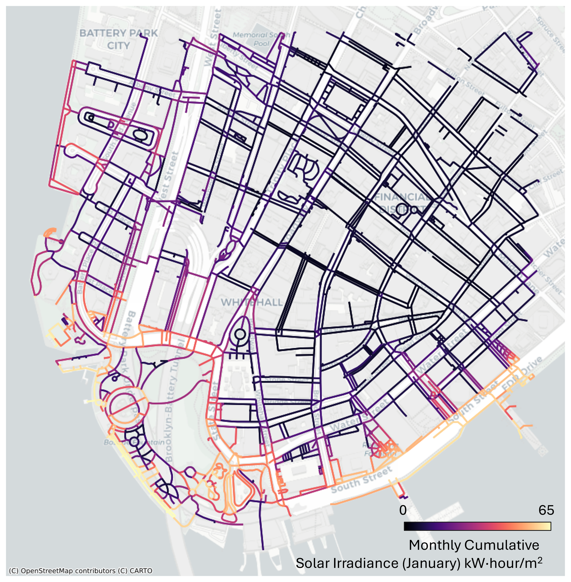
Cumulative Global Solar Irradiance (kW/m²·hour) on Road Network
Please cite the paper if you use voxcity in a scientific publication:
Fujiwara K, Tsurumi R, Kiyono T, Fan Z, Liang X, Lei B, Yap W, Ito K, Biljecki F. VoxCity: A Seamless Framework for Open Geospatial Data Integration, Grid-Based Semantic 3D City Model Generation, and Urban Environment Simulation. arXiv preprint arXiv:2504.13934. 2025.
@article{fujiwara2025voxcity,
title={VoxCity: A Seamless Framework for Open Geospatial Data Integration, Grid-Based Semantic 3D City Model Generation, and Urban Environment Simulation},
author={Fujiwara, Kunihiko and Tsurumi, Ryuta and Kiyono, Tomoki and Fan, Zicheng and Liang, Xiucheng and Lei, Binyu and Yap, Winston and Ito, Koichi and Biljecki, Filip},
journal={arXiv preprint arXiv:2504.13934},
year={2025},
doi = {10.48550/arXiv.2504.13934},
}
.png)