Atmospheric chemistry enhances climate mitigation potential of tree restoration

Natural climate solutions, including conservation, restoration and improved land management, can play a role in limiting global warming to well below 2 K above preindustrial^1,2,3. For example, large-scale tree restoration including reforestation and afforestation could help capture atmospheric carbon dioxide (CO₂) comparable to the present-day anthropogenic carbon that resides in the atmosphere^4,5,6,7. Concern over tree restoration, however, has been expressed due to several climate-related factors including increased risk of drought and wild fire activity, shifts in regional water availability, as well as to biotic factor^8,9,10,11. Furthermore, biogeophysical factors which include changes in surface energy fluxes (e.g., changes in surface albedo) can enhance or diminish the negative climate forcing associated with enhanced carbon sequestration^{12,13,14,15,16,17,18,19,20}. Complete global afforestation or deforestation can also have a significant impact on climate through changes in large-scale atmospheric and oceanic circulation²¹.

Studies have also shown the importance of atmospheric chemistry and short-lived climate forcers (SLCFs), including biogenic volatile organic compound (BVOC) impacts on aerosols, methane and ozone. For example, the net atmospheric chemistry effect associated with historical cropland expansion (accomplished in part through deforestation) is a negative climate forcing²². In contrast, a similar study that also included aerosol cloud interactions (i.e., cloud albedo effect) found that complete (global) deforestation led to an overall positive radiative forcing from SLCFs²³. Similarly, historical land use change (1850–2000) led to a small net positive SCLF radiative effect, with positive aerosol radiative effects associated with reduced biogenic SOA outweighing the negative radiative effects associated with reductions in methane and ozone²⁴. More recently, a forestation scenario with extensive global expansion in suitable regions led to a combined albedo and chemistry radiative effect that offset up to a third of the negative forcing associated with enhanced land carbon storage²⁵.

Overall, many studies utilize idealized land cover change scenarios such as global afforestation or deforestation^21,23 or focus on the radiative forcing effects^22,23,24,25. Here, we examine the full chemistry-climate response of a high-end tree restoration scenario. Two sets of Community Atmosphere Model versions 6²⁶ (CAM6) present-day (year 2000) time-slice simulations coupled to the Community Land Model version 5²⁷ (CLM5) and a slab ocean model are performed, including a tree restoration experiment and a baseline control with interactive atmospheric chemistry²⁸. An identical pair of simulations are also performed but without interactive atmospheric chemistry (Methods). Note that as standard in the current generation of climate models, methane is prescribed; however, we estimate both its direct and indirect effects via the simulated change in atmospheric oxidation. The difference between the former set of simulations is abbreviated CHEM; the difference between the latter set of simulations is abbreviated NOCHEM. The difference between these two signals (CHEM minus NOCHEM) isolates the chemistry-climate effect, which is a seldom simulated part of the biogeophysical effect. As it is difficult to quantify the effects of individual climate drivers under our experimental design, our emphasis is on the overall effects of atmospheric chemistry.

Tree restoration scenario

Figure 1 shows the change (relative to the 2000 baseline) in tree, crop, shrub and grass fraction under our tree restoration scenario (Methods; see also Supplementary Figs. 1 and 2). Global tree area increases by 12.31 Mkm², which is similar to other recent estimates of the global tree restoration potential^4,5. The increase is largely at the expense of grass (global decreases of −8.16 Mkm²) followed by crop (−4.17 Mkm²) and barren land (−0.15 Mkm²) with small increases in shrub (0.16 Mkm²). Temperate trees constitute the largest increase at 5.98 Mkm² (49%) followed closely by tropical trees at 5.57 Mkm² (45%) and then boreal trees at 0.77 Mkm² (6%). Northern Hemisphere (NH) tree restoration accounts for 66% (8.10 Mkm²) of the global increase and consists largely of temperate trees at 5.04 Mkm², followed by tropical trees as 2.31 Mkm² and boreal trees at 0.76 Mkm². Southern Hemisphere (SH) tree restoration accounts for 34% (4.21 Mkm²) of the global increase, which is dominated by tropical trees at 3.26 Mkm² followed by small increases in both temperate and boreal trees at 0.94 and 0.01 Mkm², respectively.

Fig. 1: Land fraction perturbation under global tree restoration.

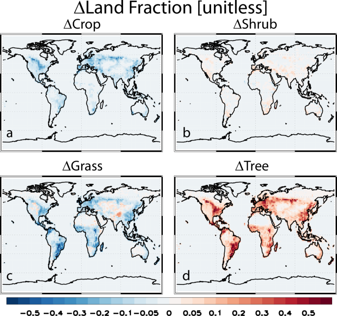
a Crop; b shrub; c grass; and d tree fraction perturbation used to drive CAM6 simulations. Units are dimensionless. Changes are relative to the baseline land use data in year 2000.

Near-surface air temperature response

Figure 2 shows the near-surface air temperature (TAS) response to tree restoration under CHEM and NOCHEM, and the corresponding effects of interactive atmospheric chemistry (CHEM minus NOCHEM). NOCHEM (Fig. 2b) simulates a global mean TAS increase of 0.19 ± 0.03 K, including more warming in the NH at 0.26 ± 0.03 K as compared to the SH at 0.11 ± 0.03 K. Regionally, the largest warming occurs in the NH temperate regions, particularly those regions with relatively large increases in tree fraction (e.g., Fig. 1d). Most of the Arctic warms under both CHEM and NOCHEM, which is likely related to the importance of the ice-albedo feedback here. Weaker and more localized cooling occurs in some SH regions (which also feature relatively large increases in tree fraction) including tropical areas such as parts of southeastern Brazil and southern Africa. Such responses are in general consistent with the notion that temperate (and boreal) trees yield annual mean warming due to surface darkening (which is exacerbated in snowy areas) whereas tropical trees yield annual mean cooling due to enhanced evapotranspiration¹⁶.

Fig. 2: Near-surface air temperature response to global tree restoration.

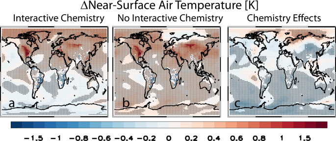
Results are based on simulations (a) with and b without interactive atmospheric chemistry. The effects of interactive atmospheric chemistry (c) are estimated as the difference (i.e., a, b). Responses are estimated from CAM6 simulations coupled to a slab ocean model over the last 150 years of the simulation (years 50–199). Black dots show changes significant at the 90% confidence level based on a standard t-test. Units are K.

When our simulations include interactive atmospheric chemistry (Fig. 2a), much of this warming is muted, especially in the SH. For example, the global mean TAS increase is reduced to 0.07 ± 0.03 K, i.e., the effects of interactive chemistry yield net global mean cooling of −0.11 ± 0.04 K (Supplementary Table 1). Although this muting effect occurs in both hemispheres, it is particularly strong in the SH where warming under NOCHEM reverses to cooling under CHEM (−0.04 ± 0.03 K). The net effect of including interactive chemistry is therefore cooling in both hemispheres, −0.06 ± 0.05 K in the NH and −0.16 ± 0.04 K in the SH. We note the regional nature of these temperature responses, as some NH regions with large increases in tree fraction (e.g., central US; eastern Europe; central Russia) warm substantially by up to 1.8 K. Similarly, some regions in the SH with large increases in tree fraction (e.g., southeastern Brazil) cool substantially by up to −1.5 K.

As with most current climate models, CAM6 with interactive chemistry constrains methane to specified surface concentrations, which limits any changes in its atmospheric concentration and its influence on climate. However, as will be discussed below, tree restoration reduces the oxidative capacity of the atmosphere, largely through enhanced emissions of BVOCs and subsequent reduction in hydroxyl radical (OH) concentrations. This in turn would increase the methane lifetime and its concentration, as well as tropospheric ozone and stratospheric water vapor. We estimate the change in methane concentration that would be expected, if it were not constrained, from the change in its lifetime due to loss via reaction with OH^29,30. The direct and indirect effect of increased methane leads to estimated global mean warming of 0.04 K (0.03 to 0.06 K), which mutes some of the aforementioned cooling effect under CHEM (Methods).

As will be discussed below, chemistry effects yield net cooling primarily due to increases in BVOC emissions and enhanced SOA, which results in decreased downwelling solar radiation (via both aerosol direct effects and cloud effects). This chemistry cooling effect is stronger in the SH as compared to the NH, which is consistent with stronger increases in BVOC emissions, including both isoprene and monoterpene emissions, as well as stronger increases in SOA burden in the SH. This response is consistent with the fact most of the tree restoration in the SH consists of tropical trees, which are the dominant emitters of most BVOCs³¹.

Surface energy balance decomposition

As our simulations are coupled to a slab ocean model and therefore include the full temperature response and the associated feedbacks, it is difficult to diagnose cause versus effect. Nonetheless, we use the surface energy balance (SEB; Methods) decomposition^32,33,34 to understand the drivers of the temperature changes above, including the differential response between CHEM and NOCHEM. Figure 3 shows the zonal mean SEB decomposition (Supplementary Fig. 3 shows maps over all land regions). Unless otherwise noted, all SEB analyses are subsampled to land areas where the tree fraction increases by at least 0.1. Thus, this analysis provides a local/regional assessment of the impacts of tree restoration. We first note that the SEB decomposition reasonably reproduces the change in surface temperature (TS) and TAS (Supplementary Fig. 4). For example, the SEB reconstructed global mean TS response under CHEM is 0.12 ± 0.04 K relative to the actual TS and TAS responses of 0.08 ± 0.04 K and 0.12 ± 0.04 K, respectively (Supplementary Table 2).

Fig. 3: Surface energy balance (SEB) decomposition of the surface temperature response.

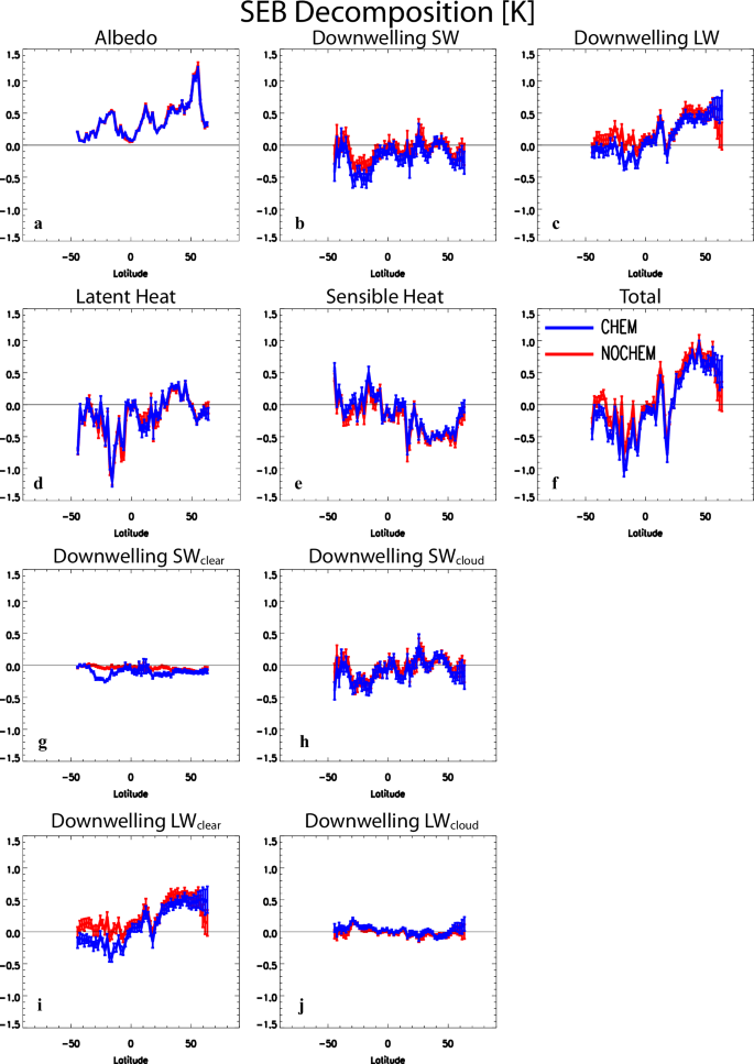
Zonal annual mean responses for a surface albedo; b downwelling surface shortwave radiation; c downwelling surface longwave radiation; d surface latent heat flux; e surface sensible heat flux; and f the total (i.e., sum of the prior five terms). Also included is the decomposition of the downwelling surface shortwave radiation term into g clear and h cloudy sky contributions and the corresponding decomposition of the downwelling surface longwave radiation term into i clear and j cloudy sky contributions. To isolate the contribution from the tree restoration perturbation, the SEB decomposition is performed over land areas where the change in tree fraction is at least 0.1. Results are based on simulations with (blue lines) and without (red lines) interactive atmospheric chemistry as estimated from CAM6 simulations coupled to a slab ocean model over the last 150 years of the simulation (years 50–199). Error bars show the 90% confidence interval. Units are K.

The surface albedo term (Fig. 3a) leads to warming at all latitudes, with two relative maxima of about 0.5 K in the NH and SH subtropics, similar NH midlatitude warming, and a warming maximum that approaches 1.5 K near 60 °N. The tree fraction increase exhibits peaks at similar latitudes (Supplementary Fig. 1d). This is consistent with the surface darkening effect of tree restoration, particularly at higher latitudes. Furthermore, the albedo term consistently contributes the most to the total warming signal, particularly in the NH (Supplementary Table 2). The large warming in the central US (Fig. 2a, b) is largely related to the large warming associated with the surface albedo term (Supplementary Fig. 3a, b). This general region has a relatively large potential albedo change (associated with the most likely open land to woody savanna/forest cover transition), which is not inconsistent with our results¹⁹. In contrast, the surface latent heat flux component of SEB (Fig. 3d) primarily yields cooling, particularly in the SH near 15–20 °S (where a large tropical tree fraction increase occurs) of about −1 K. These two terms—which are very similar between CHEM and NOCHEM—help to explain the larger warming in the NH under both signals, as well as the relatively strong localized temperature responses in some regions.

The surface downwelling shortwave (SW) radiation term (Fig. 3b) primarily contributes cooling under both signals, particularly in the SH. Furthermore, this term shows significantly more cooling under CHEM as opposed to NOCHEM. For example, the chemistry effect (CHEM minus NOCHEM) yields cooling of −0.08 ± 0.04 K in the NH which increases in magnitude to −0.15 ± 0.04 K in the SH (Supplementary Table 2). Thus, the decrease in downwelling SW radiation is a dominant driver for the reduced warming under CHEM and in particular the SH cooling under CHEM (i.e., Fig. 2). Furthermore, there are contributions under both clear-sky (SW_clear) and cloudy-sky (SW_cloud) (Fig. 3g, h; Supplementary Fig. 5). In the NH, the SW cooling under the chemistry effect is equally split between SW_clear (−0.04 ± 0.02 K) and SW_cloud (−0.04 ± 0.05 K). In the SH, this SW cooling is dominated by SW_clear at −0.10 ± 0.01 K (SW_cloud is −0.05 ± 0.05 K). As discussed below, the larger cooling from the SW term under CHEM is consistent with vegetation BVOC responses and enhanced secondary organic aerosol (SOA). This includes aerosol direct effects (e.g., scattering of solar radiation) as suggested by the enhanced SW_clear cooling under CHEM and aerosol-cloud effects as suggested by the enhanced SW_cloud cooling under CHEM.

Non-aerosol related cloud responses (Supplementary Figs. 6–10; Supplementary Table 3; Supplementary Note 1) to tree restoration^35,36 also contribute to the decrease in surface downwelling SW radiation. In the SH, for example, the SW_cloud term yields relatively large cooling under not only CHEM (−0.21 ± 0.05 K) but also NOCHEM (−0.17 ± 0.05 K). These SH SW_cloud responses are consistent with corresponding increases in low cloud cover (0.93 ± 0.15% under CHEM and 0.68 ± 0.14% under NOCHEM; Supplementary Table 3), as found using satellite data³⁶. These SH low cloud increases are consistent with moistening of the lower atmosphere, e.g., relative humidity at the model’s lowest level increases by 1.60 ± 0.15% under CHEM and 1.40 ± 0.14% under NOCHEM (Supplementary Table 3), which is consistent with the increase in latent heat flux (i.e., evapotranspiration). Note, however, that in the NH we find drying of the lower atmosphere and decreases in low cloud cover at −0.24 ± 0.11% for CHEM and −0.38 ± 0.11% for NOCHEM. The other two terms of the SEB decomposition including surface downwelling longwave radiation and sensible heat flux appear to be largely a feedback response (Supplementary Note 2).

Aerosols, cloud and ozone related responses

Figure 4 shows zonal mean plots of several aerosol related variables (Supplementary Fig. 11 shows maps). Tree restoration under CHEM yields increases in the BVOCs isoprene and monoterpene (Supplementary Table 4), largely in the SH subtropics where the large tropical tree increase occurs, and in turn, increases in chemical production of SOA (global mean increase of 1.79 ± 0.03 ng m⁻² s⁻¹ which corresponds to an 18.5% increase relative to the control; Supplementary Table 4) and SOA burden (Fig. 4a). NOCHEM does not explicitly simulate BVOCs and SOA changes are much smaller, e.g., the SOA global mean change is 0.40 ± 0.01 mg m⁻² under CHEM (corresponding to a 19% increase relative to the control) versus −0.001 ± 0.003 mg m⁻² under NOCHEM (Supplementary Table 4). In contrast to SOA increases, tree restoration yields decreases in dust burden (Fig. 4c) under both CHEM and NOCHEM, particularly in the NH (e.g., −6.5 ± 4.0 mg m⁻² under CHEM which corresponds to a −2.1% decrease). Reduced dust burden is consistent with reduced near-surface wind speeds (Supplementary Fig. 12) under tree restoration (due to enhanced surface roughness) and in turn, less dust emissions (e.g., NH dust emissions decrease by −2.5% under CHEM). There is also a hemispheric asymmetry in the sulfate (SO₄) burden response—including increases in the NH but decreases in the SH (Fig. 4b; Supplementary Note 3)—but other aerosol species show weak decreases in both hemispheres. These decreases are consistent with increases in aerosol dry deposition, again consistent with enhanced surface roughness under tree restoration (Supplementary Note 3).

Fig. 4: Aerosol, cloud and ozone related responses.

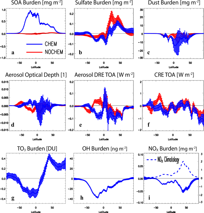
Zonal annual mean responses for a secondary organic aerosol (SOA) burden [mg m⁻²]; b sulfate aerosol burden [mg m⁻²]; c dust aerosol burden [mg m⁻²]; d aerosol optical depth (AOD; unitless); e aerosol direct radiative effect (ADRE) at the TOA [W m⁻²]; f cloud radiative effect at the TOA [W m⁻²]; g tropospheric ozone (TO₃) burden [DU]; h hydroxyl radical (OH) burden [ng m⁻²]; and nitrogen oxide (NO_x) burden [mg m⁻²]. Results are based on simulations with (blue lines) and without (red lines) interactive atmospheric chemistry as estimated from CAM6 simulations coupled to a slab ocean model over the last 150 years of the simulation (years 50–199). Error bars show the 90% confidence interval. Blue dashed line in (i) shows the annual mean NO_x climatology from the control simulation.

The offsetting dust and SOA changes help to explain the corresponding changes in aerosol optical depth (AOD; Fig. 4d) and aerosol direct radiative effect at the top-of-the-atmosphere (ADRE TOA; Fig. 4e; see also Supplementary Fig. 13). In the SH subtropics, increased AOD occurs under CHEM, whereas NOCHEM yields corresponding AOD decreases. These changes are reflected (but inverted) in ADRE TOA, i.e., CHEM yields decreases whereas NOCHEM yields increases. In the SH subtropics, AOD increases under CHEM are associated with increases in SOA that are only partially offset by decreases in sulfate and dust, while AOD decreases under NOCHEM are associated with decreases in sulfate and dust. In the NH, nonsignificant decreases in AOD occur under both CHEM and NOCHEM, generally consistent with NH dust decreases that are partially offset by increases in SOA (CHEM only) and sulfate. Both CHEM and NOCHEM, however, yield decreased ADRE TOA in the NH (consistent with SOA and SO₄ increases), with more negative and significant changes under CHEM (consistent with the much larger NH increase in SOA). Thus, increases in SOA and decreases in dust (and sulfate changes) compete in driving changes in ADRE TOA, with SOA dominating under CHEM, especially in the SH. This helps to account for the reduced warming under CHEM, including the SH cooling. As expected, similar (but larger) aerosol responses occur over land only (Supplementary Table 4).

As mentioned above, cloud responses also contribute to the reduced warming under CHEM (Supplementary Note 1; Supplementary Figs. 9 and 10). Figure 4f shows the cloud radiative effect (CRE; Methods) at TOA is generally more negative under CHEM as opposed to NOCHEM, particularly in the SH between 60 °S to 15 °S. We note that CRE over land is influenced by the tree restoration perturbation (i.e., CRE has a negative contribution over tree restoration regions due to the surface darkening effect). This issue is reduced (but not necessarily eliminated) when quantifying the chemistry effect (i.e., CHEM minus NOCHEM), and it is also not relevant over the ocean. Restricting our CRE TOA analysis to oceans only yields similar results (Supplementary Fig. 9h). In the SH, the CRE TOA response over ocean is −0.14 ± 0.12 W m⁻² under CHEM but 0.10 ± 0.11 W m⁻² under NOCHEM (Supplementary Table 3), i.e., the chemistry effect yields −0.24 ± 0.17 W m⁻². This response is consistent with an increase in SH low cloud cover under CHEM at 0.16 ± 0.10% and a corresponding decrease under NOCHEM at −0.10 ± 0.09% (Supplementary Table 3). These changes result in larger net increase in SH low cloud cover of 0.25 ± 0.12% due to the chemistry effect, largely over the SH oceans (Supplementary Fig. 6). Consistent changes also occur to cloud microphysical properties (Supplementary Fig. 10), and in particular, very clear differences between CHEM and NOCHEM exist, largely in the SH. For example, cloud condensation nuclei (CCN) and cloud water number concentration (CDNC) increase and average cloud droplet effective radius (Re) decreases in the SH under CHEM. Under NOCHEM there are opposite changes (Supplementary Table 3). These cloud microphysical responses under CHEM are consistent with the relatively large increase in SOA (i.e., aerosol-cloud indirect effects).

Tropospheric ozone burden (TO₃, defined as the burden below the 150 ppb ozone level; Fig. 4g) decreases globally (−0.034 ± 0.030 DU; −0.14% relative to the control), but with a hemispheric contrast including decreases in the SH (−0.19 ± 0.04 DU; −1.0% decrease relative to the control) and increases in the NH (0.12 ± 0.04 DU; 0.4% increase). The SH TO₃ decrease is consistent with the large increase in BVOCs (e.g., isoprene; Fig. 4a) which are oxidized by TO₃ and OH (OH burden also decreases; Fig. 4h). The NH TO₃ increase is also consistent with the (albeit weaker) increase in BVOCs (especially isoprene) under higher nitrogen oxide (NO_x) concentrations (Fig. 4i), which drives TO₃ production^23,37. Decreases in NH O₃ dry deposition may also contribute to the NH TO₃ increase (Supplementary Figs. 14l and 15l). Although the hemispheric contrast in the TO₃ (a greenhouse gas) response is qualitatively consistent with the hemispheric contrast in the near-surface air temperature response under CHEM, i.e., decreases in SH TO₃ are consistent with SH cooling and increases in NH TO₃ are consistent with NH warming, additional qualitative analysis suggests changes in TO₃ are unlikely a strong driver of the muted warming under CHEM (Supplementary Note 4; Supplementary Figs. 14 and 15). Moreover, offline radiative transfer calculations show relatively small instantaneous radiative effects associated with the ozone response (Methods). Other notable climate responses include a hemispheric contrast in precipitation including a northward tropical precipitation shift (Supplementary Fig. 16; Supplementary Note 5).

In terms of air quality (based on CHEM), surface ozone (O₃) increases globally over land, including increases over NH land and weaker decreases over SH land (Supplementary Table 4; Supplementary Fig. 17). Although these large-scale changes are relatively small (e.g., NH land increase of 0.78 ± 0.07 ppb represents a 2.2% increase relative to the control), there are much larger regional changes over the central US, eastern Europe and eastern China. For example, in the central US O₃ increases approach 6–7 ppb, which represents a 20–25% increase relative to the control. These locations correspond to very high nitrogen oxide (NO_x) levels at year 2000 and relatively large tree increases, and thus increases in BVOCs, which leads to strong increases in surface O₃. Surface fine particulate matter (PM25) exhibits less robust changes (consistent with the opposing changes of SOA and dust) including nonsignificant decreases over NH land but significant increases over SH land at 0.31 ± 0.07 μg m⁻³ (a 3.6% increase relative to the control). Again, however, there are regions associated with relatively large tree restoration that feature larger increases in PM25, including the US, Europe, eastern China and in particular southeastern Brazil. Over the latter region, for example, PM25 increases approach 5 μg m⁻³, which represent a 60–70% increase relative to the control. Thus, forested areas in the NH may experience degraded air quality (largely in terms of O₃, but also PM25). Forested areas in the SH in general have improved air quality in terms of O₃, but degraded air quality in terms of PM25 (largely over Brazil). Degraded PM25 air quality by the end of this century was also found by another study that compared ssp126 versus ssp370 land-use (associated with reduced tropical deforestation and increased afforestation), consistent with not only enhanced BVOCs and SOA, but also dust³⁸.

Fire and Land Carbon Responses

Fire carbon emissions (and fire burned area) decrease globally and in both hemispheres (more so in the SH) under both CHEM and NOCHEM (Fig. 5; Supplementary Table 5). Most of this large-scale decrease occurs in the tropics (30 °S to 30 °N), largely near Colombia/Venezuela and southeast Brazil which correspond to regions with large increases in tree fraction. NOCHEM yields a decrease in tropical fire carbon emissions of −9.9 ± 1.0 kgC km⁻² day⁻¹ (a 21.2% decrease relative to the control), with similar decreases under CHEM. These decreases are consistent with tropical near-surface relative humidity increases (i.e., 0.49 ± 0.10% under CHEM) which decreases fuel flammability, with enhanced canopy transpiration dominating over the warming (Supplementary Fig. 18), i.e., increased water vapor exceeds the increase in saturation vapor pressure. In contrast, significant increases in fire carbon emissions occur in the extratropics (e.g., central US). NH extratropical (NHE; 30–60 °N) fire carbon emissions under NOCHEM increase by 5.70 ± 0.62 kgC km⁻² day⁻¹ (a 39.0% increase relative to the control) and the corresponding SH extratropical (SHE; 30–60 °S) increase is 10.7 ± 2.7 kgC km⁻² day⁻¹ (a 23.9% increase relative to the control). These increases are consistent with decreases in extratropical near-surface relative humidity which increases fuel flammability, with both warming and transpiration decreases contributing in some regions (e.g., central US; Supplementary Fig. 18). Comparing CHEM with NOCHEM, these extratropical increases in fire carbon emissions are significantly weaker under CHEM, i.e., the chemistry effect yields net decreases at −0.87 ± 0.82 and −4.9 ± 3.6 kgC km⁻² day⁻¹ in the NHE and SHE, respectively (Supplementary Table 5). The weaker extratropical fire increases under CHEM are consistent with muted warming and less drying (e.g., the chemistry effect yields net increases in near-surface relative humidity).

Fig. 5: Fire responses to global tree restoration.

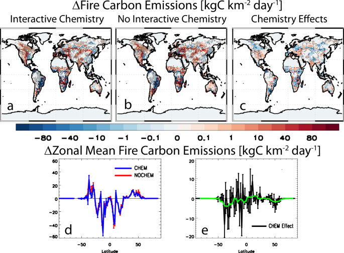
Fire carbon emissions [kgC km⁻² day⁻¹] responses based on simulations a with and b without interactive atmospheric chemistry and c their difference. Corresponding zonal mean responses for d simulations with (blue lines) and without (red lines) interactive chemistry and e their difference (CHEM Effect; green line shows smoothed values). Note the different y-scale between (d) and (e). Black dots in (a–c) show changes significant at the 90% confidence level based on a standard t-test. Error bars in (d, e) show the 90% confidence interval.

To help support the above claims, we calculate the global spatial correlation (across grid boxes) between fire carbon emissions and several climate-related variables. The corresponding correlation between fire carbon emissions and near-surface relative humidity responses is −0.28 for CHEM and −0.27 for NOCHEM (both significant at the 99% confidence level). These correlations are weaker when near-surface air temperature is used at 0.19 and 0.23, respectively. Although decreases in near-surface wind speeds (Supplementary Fig. 12) could be important to the fire carbon emissions response in some regions (e.g., the decrease in tropical fire carbon emissions), the global spatial correlation between fire carbon emissions and near-surface wind speed responses is also weaker at 0.18 for CHEM and 0.16 for NOCHEM. Similarly, weaker correlations exist between fire carbon emissions and soil water in the top 10 cm at −0.07 for CHEM and −0.06 for NOCHEM. We also note that the broad fire changes discussed above (decreases in the tropics and increases in the extratropics) may also be related to the land cover change. Tropical tree restoration generally replaces grasses, whereas extratropical tree restoration (particularly in the NH) replaces a mixture of both grass and crop (Fig. 1). As grasses are in general more flammable compared to forest and crop, replacing grasses with less flammable trees in the tropics may subdue fire activity. In contrast, replacing crop with trees in the extratropics may enhance fire activity. This is supported by the fact fire burned area increases in the extratropics (Supplementary Table 5), despite the (expected) decrease in fire burned area for crops (Supplementary Table 5).

The decrease in tropical fire carbon emissions under both CHEM and NOCHEM suggests the enhanced carbon sequestration associated with tropical tree restoration in our simulations is not counteracted by enhanced fire activity. However, the opposite is true for the extratropics, where some of the enhanced carbon sequestration will be lost due to increased fire carbon emissions. This is particularly true under NOCHEM, where the increase in NHE fire carbon emissions drives ~20% of the decrease in net primary productivity (NPP; Supplementary Table 5). We reiterate that our simulations are time-slice experiments that feature fixed atmospheric CO₂ concentrations. Thus, the above statements do not include the impact of continued anthropogenic warming, which is likely to exacerbate fire weather across most burnable land areas³⁹.

Land carbon (which is the sum of vegetation, litter and soil organic matter carbon) increases over the course of the simulation (Fig. 6a–c), largely in the first year, which is consistent with the instantaneous increase in trees (maps are included in Supplementary Fig. 19). Note that the land carbon pools are not yet in equilibrium and the biogeophysical effects are still developing. Most of the increase is due to vegetation carbon (i.e., stems, leaves and roots), followed by soil organic matter and litter carbon (Fig. 6d–l; Supplementary Table 6). In the first decade, the SH sequesters 43% of the global land carbon, despite representing only 34% of the global tree area increase. This is consistent with the fact most of the SH tree restoration occurs in the tropics, which contain more carbon dense trees. The enhanced carbon storage in the SH is also evident over the course of the simulation. By the last decade, the SH is responsible for 48% of the global land carbon storage. Normalizing the NH and SH land carbon increase in the last decade by the corresponding increase in hemispheric tree area yields land carbon storage efficiencies under CHEM of 13.6 ± 0.06 and 23.8 ± 0.06 PgC per Mkm² in the NH and SH, respectively (NOCHEM yields corresponding values of 12.6 ± 0.05 and 22.5 ± 0.11 PgC per Mkm², respectively). This implies SH tree restoration (and more specifically tropical tree restoration) under our scenario yields more efficient carbon storage (by a factor of 1.75 compared to the NH).

Fig. 6: Land carbon time series.

Global annual mean (a–c) vegetation + litter + soil organic matter carbon; (d–f) vegetation carbon; (g–i) litter carbon; and (j–l) soil organic matter carbon responses for the (a, d, g, j) Northern Hemisphere; (b, e, h, k) Southern Hemisphere; and (c, f, i, l) globe. Results are based on simulations with (blue lines) and without (red lines) interactive atmospheric chemistry as estimated from CAM6 simulations coupled to a slab ocean model. Units are PgC.

Another contributing factor to the hemispheric difference in carbon storage is a larger SH increase in soil organic matter carbon (Fig. 6j–l; 12.4 ± 0.12 PgC in the SH versus 0.23 ± 0.10 PgC in the NH under CHEM). We note some NH regions, in particular the central US, feature decreased carbon storage (and decreased NPP) despite tree increases (Supplementary Fig. 19m–o). In addition to the previously discussed fire increase here, this may be related to the model’s dry precipitation bias in this region²⁶, which may lead to unrealistic restrictions on tree growth. For example, re/afforestation of the central US (also using CESM2) did not support strong tree growth, as this region exhibited small or no carbon gains⁴⁰. We also note that the central US features a transition from crops to trees (e.g., Supplementary Fig. 2), which may decrease productivity.

The chemistry effect yields net increases in all three carbon pools (Fig. 6), with total land carbon increasing by 13.0 ± 0.91 PgC, which represents a 6.6% increase relative to NOCHEM. Interestingly, the chemistry effect yields larger increases in the NH (as compared to the SH) for all three carbon pools. Similar statements apply to NPP, where the chemistry effect yields net increases globally at 6.2 ± 3.0 kgC km⁻² day⁻¹, largely due to NH increases at 8.1 ± 4.3 kgC km⁻² day⁻¹ (Supplementary Table 5). The enhanced carbon sink (and carbon fixation) under CHEM is consistent with the weaker increase in extratropical fire carbon emissions previously discussed. Most of it, however, appears to be related to increases in nitrogen deposition (which cannot change under NOCHEM), consistent with enhanced surface roughness associated with tree restoration. For example, nitrogen deposition under CHEM increases globally at 12.1 ± 0.7 gN km⁻² day⁻¹, and this is largely due to NH increases at 16.9 ± 1.2 gN km⁻² day⁻¹, with weaker SH increases at 2.2 ± 1.4 gN km⁻² day⁻¹ (Supplementary Table 5; Supplementary Fig. 19p–r). The larger NH increase is because there is more atmospheric nitrogen in the NH as compared to the SH. The global spatial correlation (across grid boxes) between nitrogen deposition and land carbon responses is 0.51 (0.47 if NPP is used; both of these correlations are significant at the 99% confidence level).

The transient climate response to cumulative CO₂ emissions (TCRE) represents a near-linear relationship between cumulative anthropogenic CO₂ emissions and global warming since the preindustrial, and provides a good first estimate of the near-surface air temperature response to land carbon changes^41,42,43. CESM2 yields a TCRE of 2.13 K per 1000 PgC⁴³. We note that this is on the high end of TCRE estimates, as the best estimate is 1.65 K per 1000 PgC, with a likely range from 1.0 to 2.3 K per 1000 PgC⁴⁴. Using the CESM2 TCRE value, along with the increase in land carbon storage over the last 10 years of the simulations (years 190–199; Supplementary Table 6), both CHEM and NOCHEM yield similar estimates for the global mean cooling effect associated with enhanced land carbon storage at −0.45 K under CHEM versus −0.42 K under NOCHEM. Thus, despite the larger total land carbon storage under CHEM, the chemistry effect on land carbon storage yields small cooling at −0.03 K. We note that using the TCRE to estimate the biogeochemical cooling effect is an approximation. Future studies should pursue emissions driven simulations to more accurately estimate the draw-down in atmospheric CO₂ associated with the enhanced carbon storage of tree restoration, and the corresponding impacts on temperature and climate.

We conclude by noting that our results are based on a single model. Furthermore, our tree restoration is instantaneous imposed, so we are unable to quantify the transient climate evolution in response to a more realistic tree afforestation/reforestation (e.g., where trees are added incrementally through time). Future studies with alternative models and more realistic transient tree restoration should be performed to evaluate the robustness of the results found here. Furthermore, emissions-based simulations should also be pursued, so that the biogeochemical effects of tree restoration are explicitly simulated. Nonetheless, our results show that tree restoration leads to global mean cooling due to enhanced carbon sequestration (as approximated by the TCRE). This cooling, however, is muted due to biogeophysical effects, largely associated with surface darkening. Biogeophysical effects mute 45% of the biogeochemical cooling under NOCHEM (0.19 K versus 0.42 K, respectively). In contrast, biogeophysical effects mute 16% of the biogeochemical cooling under CHEM (0.07 K versus 0.45 K, respectively), which increases to 24% when methane effects are accounted for (0.11 K versus 0.45 K, respectively). Thus, including interactive chemistry yields larger net cooling under tree restoration.

The enhanced cooling associated with the chemistry effect is largely associated with enhanced SOA and cloud effects. Using the SEB decomposition (which provides a local/regional perspective as we subsample to grid boxes with an increase in tree fraction of at least 0.1), the dominant driver for the reduced warming under CHEM and in particular the SH cooling is a larger decrease in downwelling SW radiation, with contributions under both clear-sky and cloudy-sky. The SEB analysis also yields SH SW_cloud cooling under both CHEM and NOCHEM, consistent with increased low cloud cover under both frameworks (and the observational-based study of ref. ³⁶). Furthermore, increased evapotranspiration (i.e., the latent heating term) is important to SH cooling under both CHEM and NOCHEM. This increase is consistent with moistening of the lower atmosphere, which in turn is consistent with the increase in low cloud cover.

Taking a broader perspective (i.e., not subsampled), increases in SOA under CHEM, especially in the SH, are consistent with a larger negative aerosol DRE TOA. Furthermore, the CRE TOA is generally more negative under CHEM as opposed to NOCHEM, particularly in the SH. This is consistent with an increase in SH low cloud cover under CHEM and a corresponding decrease under NOCHEM. Consistent changes also occur to cloud microphysical properties. For example, CCN and CDNC increase and Re decreases in the SH under CHEM. Under NOCHEM there are opposite changes. These cloud microphysical responses under CHEM are consistent with the relatively large increase in SOA (i.e., aerosol-cloud indirect effects).

The lack of SH warming under CHEM and the importance of clouds, is also supported by analogous fixed sea-surface temperature/sea ice simulations (Methods). Figure 7 shows the NH and SH effective radiative forcing (ERF), the instantaneous radiative forcing (IRF) as estimated from the surface albedo radiative kernel and the total rapid adjustment (RAP_ADJ = ERF minus IRF). In the NH both CHEM (Fig. 7a) and NOCHEM (Fig. 7b) yield a similarly significant positive ERF (0.18 ± 0.10 W m⁻²), which is indicative of warming. This is largely associated with the significant positive IRF (i.e., due to surface darkening) at 0.23 ± 0.02 W m⁻² for both CHEM and NOCHEM. In the SH, however, notable differences exist between CHEM (Fig. 7c) and NOCHEM (Fig. 7d). In particular, CHEM yields a negligible ERF (0.01 ± 0.10 W m⁻²), which becomes weakly negative for the land surface corrected ERF (ERF_TS_ADJ) at −0.03 ± 0.10 W m⁻². This weak ERF is due to the relatively large negative total rapid adjustment (−0.11 ± 0.10 W m⁻²), which offsets the (weaker) positive IRF (0.09 ± 0.01 W m⁻²). Using radiative kernels (Methods) to decompose the total rapid adjustment into its components (Fig. 7e–h) shows that the relatively large negative total rapid adjustment in the SH under CHEM (Fig. 7g) is due to the cloud adjustment. This result is consistent across two methods, including the kernel difference method (−0.15 ± 0.09 W m⁻²) and the ISCCP simulator combined with the ISCCP radiative kernel (−0.12 W m⁻²). These independent results support the hemispheric contrast in near-surface temperature responses between CHEM and NOCHEM (i.e., CHEM yields SH cooling), while also supporting the importance of clouds to this signal.

Fig. 7: ERF, ERF_TS_ADJ, IRF and RAP_ADJ from fixed SST simulations.

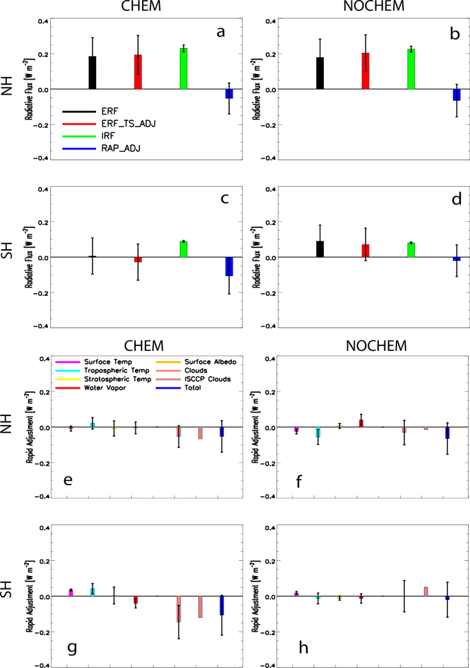
Annual mean TOA effective radiative forcing (ERF), land surface corrected ERF (ERF_TS_ADJ), instantaneous radiative forcing (IRF), and total rapid adjustment (RAP_ADJ) under (a, c) CHEM and (b, d) NOCHEM for the (a, b) NH and (c, d) SH. Annual mean TOA surface temperature, tropospheric temperature, stratospheric temperature, water vapor, surface albedo, cloud and total adjustment under (e, g) CHEM and (f, h) NOCHEM for the (e, f) NH and (g, h) SH. Error bars show the 90% confidence interval. The cloud adjustment is shown for both the kernel difference method (light pink) and that estimated from the ISCCP simulator combined with the ISCCP radiative kernel (dark pink). Units are W m⁻².

Our finding of enhanced cooling due to atmospheric chemistry effects (associated with aerosols) is in general consistent with prior studies that focused on the radiative forcing effects of SLCFs under tree de/afforestation. For example, ref. ²⁵ showed that a forestation scenario led to a negative chemistry radiative effect dominated by aerosols (with smaller, opposite signed ozone and methane radiative effects). However, unlike our SH results, their negative aerosol forcing was not large enough to offset the positive forcing associated with surface darkening. They also find a small radiative effect from clouds. A net positive radiative forcing due to SLCFs (dominated by aerosols) under deforestation²³, as well as under historical land use change (also associated with deforestation)²⁴. Both results imply a net negative forcing under afforestation. We also note that such studies focused on the radiative forcing effects alone do not address all of the climate aspects of tree restoration. For example, they do not directly account for changes in evapotranspiration, which we show here are quite important (especially in the SH)—both in terms of driving direct surface cooling, but also potentially indirect cooling through cloud impacts.

We have shown strong hemispheric asymmetries in response to tree restoration, due in part to chemistry effects. This includes stronger climate mitigation in the Southern Hemisphere (due to tropical trees), despite SH tree restoration representing only 1/3 of the global tree area increase. Moreover, increasing tropical trees is not associated with an increase in tropical mean wildfire activity. Nonetheless, our results imply larger climate benefits from afforestation and reforestation of tropical forests, particularly in the Southern Hemisphere forests of South America and southern Africa.

To conclude, our main finding is that including interactive chemistry yields larger net cooling under tree restoration. This is due to muted biogeophysical warming, largely associated with enhanced SOA and cloud effects. As the atmospheric chemistry effects of tree restoration are usually not considered, this implies higher climate change mitigation potential of tree restoration.

CAM6 simulations

We perform 1.9° × 2.5° horizontal resolution simulations with 32 vertical atmospheric levels using the Community Earth System Model version 2²⁶ (CESM2), including the Community Atmosphere Model version 6 (CAM6), the Community Land Model version 5²⁷ (CLM5) and a slab ocean model⁴⁵ integrated with the dynamic sea ice model, the Community Ice CodE version 5⁴⁶ (CICE5). Our simulations use diagnostic CO₂ (i.e., atmospheric CO₂ concentrations are prescribed as opposed to emissions-driven) and thus do not include the two-way land-atmosphere carbon cycle feedbacks. This requires the biogeochemical temperature effects associated with enhanced land carbon storage to be estimated offline using the TCRE. CLM5 is run with prognostic (but not dynamic) vegetation, active biogeochemistry (i.e., land carbon cycle) and prognostic fires including agricultural, deforestation, non-peat and peat fires^47,48. Vegetation distributions (natural plant functional types and crop functional types) are specified through time (here they are fixed) using a land use time series file, but vegetation physiology (e.g., leaf area index, canopy height) is prognostic. CLM’s fire module simulates burned area and carbon emissions, but the associated biomass burning aerosol/precursor gas emissions are not simulated here. Fire occurrence depends on ignitions, fire suppression, fuel load, and fuel combustibility^47,48,49. Ignition is parameterized as a function of lightning frequency (prescribed from observations) and population density—both of which are identical in our simulations. Fuel load is determined by the amount of all types of vegetation and litter present in a grid cell. Fuel combustibility is a function of soil moisture and relative humidity, and fire spread depends on wind speed. Socioeconomic factors (population and gross domestic product) are also used in the CLM fire parameterization, but these factors do not change in (and between) our simulations. Burned area for agricultural fires is based on an equation that includes a socioeconomic factor, fuel availability factor, fire seasonality and the area of cropland (Eq. 1 in ref. ⁴⁸). Burned area for deforestation fires is based on an equation that includes the effects of decreased tree fraction and climate conditions (Eq. 5 in ref. ⁴⁸). Since each of our simulations features fixed (i.e., non-transient) land cover (based on the tree restoration perturbation in the experiment and the year 2000 land cover data in the control), there are no deforestation fires. However, the decrease in crop fraction between the experiment and control (Fig. 1) will promote a decrease in fire burned area for cropland (Supplementary Table 5). Although CLM5 includes an optional parameterization⁵⁰ that accounts for ozone damage to vegetation (e.g., by impacting photosynthesis and stomatal conductance), our simulations do not include it. CLM5 also includes a prognostic representation of the terrestrial nitrogen cycle and its coupling to land carbon cycle. This includes the Leaf Utilization of Nitrogen for Assimilation (LUNA) module which accounts for environmental impacts on photosynthetic capacity and the Fixation and Uptake of Nitrogen (FUN) module which accounts nitrogen availability impacts on plant productivity²⁷.

CAM6 uses the Modal Aerosol Model with 4 modes (MAM4) to represent sulfate, primary and aged black carbon and organic matter, secondary organic aerosols, sea salt, and dust⁵¹. Simulations are run separately with (CHEM) and without (NOCHEM) interactive chemistry. Interactive chemistry simulations use the Model for Ozone and Related chemical Tracers (MOZART) Troposphere Stratosphere (TS1) chemistry mechanism²⁸. MOZART TS1 includes 221 gas phase and aerosol species and 528 chemical and photochemical reactions, along with a volatility basis set (VBS) parameterization for the formation of secondary organic aerosols⁵² which generates gas-phase SOA precursors with a range of volatilities resulting from the oxidation of the aromatic species, terpenes, and isoprene. Updates to the tropospheric mechanism include expansion of the isoprene oxidation scheme, dividing lumped aromatics and terpenes into individual species including improving their oxidation scheme, and updated organic nitrates. Biogenic emissions, including isoprene, monoterpene and other BVOCs, are simulated online based on atmospheric conditions (e.g., temperature, CO₂) and land cover using the Model of Emissions of Gases and Aerosol from Nature (MEGAN) v2.1³¹. We note that MEGAN v2.1 includes the dependence of BVOC emissions on light and temperature, as well as inhibition of isoprene emissions based on atmospheric CO₂ concentrations, and we acknowledge that CESM2 tends to yield a relatively strong BVOC response under 1% per year CO₂ simulations⁵³. Simulations with interactive chemistry explicitly simulate nitrogen deposition which is used by CLM5 for carbon-nitrogen cycling²⁸. In contrast, NOCHEM nitrogen deposition fluxes come from a fixed monthly climatology based on the control year (2000) and thus cannot change. Furthermore, SOA in NOCHEM is formed from the partitioning of a single lumped semi-volatile organics gas-phase species called “SOAG”⁵⁴. Fixed mass yields of condensable organic vapor (i.e., SOAG) from 5 VOC categories of the MOZART-4 gas-phase chemical mechanism⁵⁵ are assumed. MAM then calculates condensation/evaporation of the SOAG to/from several aerosol modes. Thus, NOCHEM does not simulate changes in BVOC emissions and their impact on SOA. We note that dust emissions are tuned down in CHEM (to constrain the dust optical depth in the default CAM-chem setup) through the parameter “dust_emis_fact” (i.e., dust_emis_fact = 0.26 in CHEM whereas dust_emis_fact = 0.70 in NOCHEM). Although the global mean decrease in dust emissions is larger in CHEM at −0.013 ± 0.004 μg m⁻² s⁻¹ as compared to NOCHEM at −0.006 ± 0.002 μg m⁻² s⁻¹, the former represents a smaller percentage change (relative to its control) at −3.3% for CHEM versus −4.6% for NOCHEM.

Slab ocean simulations use the full dynamic sea ice model (CICE5) and a spatially and temporally prescribed ocean heat flux and mixed layer depth, which ensures replication of realistic sea surface temperatures and ice distributions for the present climate^56,57. Slab ocean model forcing data from 50 years of a spun-up CESM2 preindustrial simulation are used, similar to the procedure in ref. ⁵⁸.

Simulations are performed under land-use/land cover conditions and atmospheric greenhouse gas concentrations and aerosol/precursor gas emissions for the year 2000 (referred to as the baseline or control). Initial land carbon pools for the year 2000 come from a previously integrated historical simulation. An analogous set of simulations (i.e., the perturbation or experiment) are performed where the default land use data set is replaced with our tree restoration scenario. A control and a perturbed simulation are separately performed with and without interactive chemistry. Simulations are integrated for 200 years, the last 150 of which are used to quantify climate responses (unless otherwise noted). Thus, the first 50 years are regarded as spin-up, which is typical for slab ocean model equilibrium, and in agreement with leveling off of the global mean near-surface air temperature time series after 50 years. Our relatively long simulations allow for better quantification of the forced signal relative to internal climate variability. Note that the land carbon pools (e.g., Fig. 6) are not yet in equilibrium and the biogeophysical effects are still developing. However, we also note that our results are not sensitive to the analysis time period. Over years 100–199 for example, the near surface air temperature responses under CHEM are 0.16 ± 0.04 K in the NH; −0.06 ± 0.04 K in the SH; and 0.05 ± 0.04 K globally.

We note that CESM2 has a relatively high equilibrium climate sensitivity at 5.15 K relative to other CMIP6 models (3.86 K with a 1-sigma range of 1.10 K)^59,60. Our results (e.g., temperature response to our tree restoration perturbation) may therefore be on the high-end as compared to other models. On the other hand, CESM2 also possesses a relatively high historical aerosol effective radiative forcing at −1.34 W m⁻² but this essentially lies within the 1-sigma uncertainty range from 20 CMIP6 models⁶¹, as well as within the 1-sigma range from observational constraints⁶².

As our simulations include the temperature (and climate) response to tree restoration, it is more difficult to isolate cause versus effect (i.e., forcing versus response) as compared to the fixed sea surface temperature experimental design where the total effective radiative forcing and that due to individual drivers can be estimated (where it is then assumed an invariant climate feedback responds to the forcing to drive surface temperature changes). Our intent here is to directly compare and quantify the climate response (including temperature feedbacks) to tree restoration with and without interactive chemistry. Thus, although we are not easily able to isolate the effects of individual climate drivers (e.g., aerosols, ozone), we are able to isolate the overall chemistry-climate effect, including biogeophyscial effects (e.g., surface energy fluxes) and atmospheric chemistry effects. Nonetheless, we do attempt to quantify the contribution of individual drivers when possible, but these will also include feedbacks to some extent. For example, we use double radiation calls to estimate the aerosol direct radiative effect (ADRE), i.e., \(\Delta \left(F-{F}_{{clean}}\right)\) where Δ is the difference between tree restoration experiment and control, F is the top-of-the-atmosphere or surface net radiative flux, and \({F}_{{clean}}\) is the same flux but neglecting the scattering and absorption by aerosols⁶³. Similarly, we estimate the cloud radiative effect (CRE) as \(\Delta \left({F}_{{clean}}-{F}_{{clear},{clean}}\right)\) where \({F}_{{clear},{clean}}\) is the flux neglecting scattering and absorbing by aerosols and clouds. The cloud radiative effect, in addition to the influence from feedbacks, is also influenced by the tree restoration perturbation (i.e., CRE has a negative contribution over tree restoration regions due to the surface darkening effect). This issue is reduced (but not necessarily eliminated) when quantifying the chemistry effect (i.e., CHEM minus NOCHEM), and it is also not relevant over the ocean. This issue does not impact the aerosol direct radiative effect (but again, it could be influenced by feedbacks).

We emphasize that our tree restoration perturbation is instantaneously imposed. Our simulations therefore do not include the temporal evolution of more realistic tree reforestation/afforestation (i.e., trees are not added incrementally through time). Instead, we focus on a biophysical upper limit of tree restoration, as discussed in the next section.

Tree restoration scenario

In CLM5, a grid cell can have a different number of fractional landunits including vegetated, lake, urban, glacier, and crop (the sum of which has to be 1.0). Furthermore, each landunit can have a different number of columns, and each column can have multiple patches each with a specific plant functional type (PFT) or crop functional type (CFT). For the vegetated landunit, there is only one column (soil) and its associated PFTs include trees, grasses, shrubs as well as barren land²⁷. CLM5 has eight different tree PFTs, including for example needleleaf evergreen temperate and broadleaf deciduous tropical. PFTs must also sum to 1.0 for each vegetated landunit (and CFTs for each crop landunit). Total tree fractional area at a grid cell is obtained by multiplying the vegetated landunit by the total tree PFT (summed over the 8 tree PFTs). Total crop fractional area at a grid cell is the same as the crop landunit.

Our tree restoration scenario is based on a 3-step process (Supplementary Fig. 2) that seeks to maximize the tree restoration potential. The first step (reforestation) is to compare the 1850 total tree PFT on the vegetated landunit at each grid cell to that in the baseline year of 2000. If the 1850 total tree PFT (summed over the 8 tree PFTs) for a grid cell is larger than that in 2000, the 1850 vegetated landunit PFTs replace those in the 2000 baseline land use data set. The assumption here is that forested areas that once existed in 1850 can be reforested. This includes areas deforested since the industrial revolution, but not those areas cleared for cropland (since crop is not changed) or urbanized land. This results in a global tree area increase (relative to the 2000 baseline) of 4.08 Mkm² (1.96 Mkm² in the NH versus 2.12 Mkm² in the SH), largely at the expense of grass area (decreases by −3.91 Mkm²), followed by barren land area (−0.25 Mkm²), with small increases in shrub area (0.08 Mkm²). Spatial maps of the change in shrub, grass, crop and tree fraction from step one (reforestation) are included in Supplementary Fig. 2a–d.

The second step (reforestation + afforestation) builds off the first step and is performed similarly, but here we iteratively loop over eight different land use projections⁶⁴ from the Shared Socioeconomic Scenarios (SSPs), including SSP1-1.9, SSP1-2.6, SSP2-4.5, SSP3-7.0, SSP4-3.4, SSP4-6.0, SSP5-3.4 and SSP5-8.5. If an SSP at the end of this century (year 2100) has a larger total tree PFT (again, summed over the 8 tree PFTs) at a grid cell than currently exists from step 1, the SSP’s vegetated landunit PFTs replace the current values. Here, the assumption is that if an SSP indicates the total tree PFT can increase at a grid cell (i.e., afforestation), then we use it. We note that we do not have internal consistency with a specific SSP, since we choose the SSP at a given grid cell that has the largest total tree PFT increase. This results in an additional increase in tree area, including a global tree area increase (relative to the 2000 baseline) of 7.07 Mkm² (4.00 Mkm² in the NH and 3.07 Mkm² in the SH). These changes are again largely at the expense of grass area (decreases by −6.77 Mkm²) followed by barren land area (−0.35 Mkm²) with small increases in shrub area (0.04 Mkm²). In terms of net change relative to step one, global tree area increases by 3.0 Mkm² (2.04 Mkm² in the NH and 0.95 Mkm² in the SH). Spatial maps of the change in shrub, grass, crop and tree fraction from step two (reforestation + afforestation) are included in Supplementary Fig. 2e–h.

As a final step (reforestation + more aggressive afforestation) that was explored but not adopted, we again iteratively loop over the eight SSPs and compare their crop fractional area in 2100 relative to that in the default 2000 baseline land use data set (which is the same as that from step #1 and #2 since crop has not changed). When an SSP has a decrease in crop fractional area at a grid box in 2100 (relative to 2000), we replace the current crop fractional area with that from the SSP. Here, crop area will decrease, but consistent with an SSP (but again, not with any particular SSP). The decrease in the crop fractional area is then used to increase the vegetated fractional area by the same amount (i.e., if crop fractional area decreases by 0.2, the vegetated fractional area is increased by 0.2). Note that this will increase the area of all PFTs (trees, as well as grasses, shrubs and barren land) on the vegetated landunit. This process results in an increase in tree area, including a global tree area increase (relative to the 2000 baseline) of 9.21 Mkm² (5.70 Mkm² in the NH and 3.51 Mkm² in the SH). These changes are again largely at the expense of grass area (decreases by −4.78 Mkm²) followed by crop area (−4.46 Mkm²) and barren land area (−0.14 Mkm²) with small increases in shrub area (0.17 Mkm²). In terms of net change relative to step two, global tree area increases by 2.14 Mkm². Note that grass (and shrub) area increases relative to step #2, with a relatively large global grass area increase of +1.99 Mkm². This is a consequence of increasing the entire vegetated landunit by the decrease in the crop landunit. Spatial maps of the change in shrub, grass, crop and tree fraction from this non-adopted step (reforestation + more aggressive afforestation) are included in Supplementary Fig. 2i–l.

Our final step (reforestation + more aggressive afforestation) that was adopted is similar to the above, but with an additional modification to maximize a tree increase (and not unintentionally increase grasses and shrubs). As before, if an SSP features an end-of-century decrease in a crop fractional area at a grid cell (relative to 2000), we replace the current crop fractional area with the SSP’s value and increase the vegetated fractional area by the same amount. Here, however, we assume that the decrease in the crop fractional area represents an upper bound by which the vegetated fractional area and the total tree PFT (summed over the 8 tree PFTs) can be increased when possible (i.e., the sum of the tree PFTs cannot exceed 1.0). Tree PFTs are increased in proportion to their current types. To compensate the increase in tree PFTs, grass PFTs are first decreased if possible (i.e., the sum of the grass PFTs cannot be negative); followed by shrub PFTs if possible; and finally followed by the barren land PFT. This is only performed if trees currently exist and if they can be increased (i.e., 0.0 < sum of tree PFTs < 1.0). To illustrate, if the crop fractional area decreases by 0.2 in an SSP in 2100 (relative to the 2000 baseline), we attempt to increase both the vegetated fractional area by up to 0.2 (at the expense of the crop) and in particular, the total tree PFT by up to 0.2. If trees already occupy, e.g., 0.9 of the vegetated landunit, we increase the total tree PFT (and the vegetated fractional area) by only 0.1 (and decrease the crop fractional area by only 0.1). To compensate, the total grass PFT is decreased by 0.1 if possible (i.e., total grass PFT cannot be negative). If the total grass PFT can be decreased by less than 0.1 (e.g., 0.05), we attempt to decrease the total shrub PFT by the remaining 0.05, followed by the barren land PFT if necessary. If the total tree PFT is 0.0 (or 1.0) no changes are made (i.e., we do not attempt to afforest treeless areas). This final step (more aggressive afforestation)—which assumes end of century SSP crop decreases are used to maximize tree increases—results in a global tree area increase (relative to the 2000 baseline) of 12.31 Mkm² (8.10 Mkm² in the NH and 4.21 Mkm² in the SH). These changes are again largely at the expense of grass area (decreases by −8.16 Mkm²) followed by crop area (−4.17 Mkm²) and barren land area (−0.15 Mkm²) with small increases in shrub area (0.16 Mkm²). In terms of net change relative to step two, global tree area increases by 5.24 Mkm² (4.10 Mkm² in the NH and 1.14 Mkm² in the SH). This final perturbation represents our high-end tree restoration perturbation. Spatial maps of the change in shrub, grass, crop and tree fraction from this adopted final step (reforestation + more aggressive afforestation) are included in Supplementary Fig. 2m–p.

Methane Effects

CAM6 with interactive chemistry²⁸ constrains methane to specified surface concentrations, which limits any changes (e.g., through changes in oxidizing capacity) in its atmospheric concentration. However, it is possible to diagnose the change in methane concentration that would be expected, if it were not constrained, from the change in its lifetime:

where C is the atmospheric methane concentration, τ is the total methane lifetime including soil loss and f is the feedback of methane on its own lifetime with a value of 1.30 ± 0.07^29,30. Given a C of 1775 ppb (representative of 2000 methane concentrations), a τ of 8.51 days in our year 2000 control simulation with interactive chemistry and a corresponding Δτ of 0.348 days, we estimate an increase in the change in methane concentration from 89.3 to 99.5 ppb. We have verified that the above quoted Δτ from our default slab ocean model simulations is similar to that obtained from analogous climatologically fixed sea surface temperature/sea ice simulations (i.e., the corresponding Δτ is 0.343).

The effective radiative forcing (ERF) from the change in methane concentration is calculated according to ref. ⁶⁵, which is scaled downwards by 0.8 to account for methane shortwave absorption impacts on rapid adjustments^66,67, and then subsequently scaled by 1.52 to account for the additional chemical production of ozone and stratospheric water vapor³⁰, i.e., total scaling is 1.22. This yields a corresponding ERF of 0.049 to 0.054 W m⁻². We use a simple approximation to calculate the near-surface air temperature response, ΔTAS=λ*ΕRF, where λ is the climate sensitivity parameter. Using an equilibrium climate sensitivity of 3 K with a 1-σ uncertainty range of 2.6 to 3.9 K⁶⁸ and a 2xCO₂ ERF of 3.52 W m⁻² with a 1-σ uncertainty range 0.36 W m⁻² (ref. ⁶⁰), λ has a best estimate of 0.85 (0.67 to 1.23) K per W m⁻². We arrive at an approximate global mean temperature change associated with changes in methane of 0.04 (0.03 to 0.06) K.

Surface Energy Balance (SEB) Decomposition

The SEB decomposition^32,33,34 is used to infer the contribution of changes in energy fluxes to changes in surface temperature (ΔTS):

where ε is the surface emissivity assumed to be 0.97³⁴, σ is the Stefan-Boltzmann constant with a value of 5.67 × 10⁻⁸ W m⁻² K⁻⁴, and TS_control is the surface temperature from the control experiment. The first term in square brackets represents the contribution from changes in downwelling surface shortwave radiation (ΔRSDS) which is multiplied by the monthly mean climatology of (1-α); the second term represents the contribution from changes in surface albedo (Δα) which is multiplied by the monthly mean RSDS climatology (changes in albedo impact upwelling surface shortwave radiation); the third term represent the contribution from changes in downwelling surface longwave radiation (ΔRLDS); the fourth term represents the contribution from changes in surface latent heat flux (ΔLH); and the final term represents the contribution from changes in surface sensible heat flux (ΔSH). We also decompose the first term on the right (i.e., the surface downwelling SW radiation term) into the contribution from changes in surface downwelling shortwave radiation under clear-sky and cloudy-sky. The clear-sky contribution is estimated as \(\Delta {{RSDS}}_{{clear}}\left(1-\alpha \right)\), where \(\Delta {{RSDS}}_{{clear}}\) is the change in clear-sky downwelling surface solar radiation. The cloudy-sky contribution is estimated as the residual between the all-sky and clear-sky SW radiation SEB components. A similar decomposition is performed for surface longwave radiation. We note that the SEB decomposition does not account for all factors, including for example the ground heat flux and changes in subsurface heat storage (both of which are assumed to be zero here), or changes in surface emissivity.

We compare the SEB estimated change in surface temperature to that simulated in our climate model experiments. In CESM2, the simulated TS is calculated at a displacement level as defined by the displacement height and roughness length³⁴. We also compare the SEB estimated change in surface temperature (ΔTS) to the more commonly used change in near-surface air temperature (ΔTAS) as simulated by CESM2. Near-surface air temperature in CESM2 is calculated at a height of two meters above the displacement level, by interpolating between the surface temperature and the air temperature of the lowest atmospheric level. Thus, there are differences in the height at which these various temperatures are estimated/simulated, which may impact the magnitude of the temperature change under tree restoration. For example, the local effects of deforestation (i.e., at the location of deforestation) have stronger impacts on surface temperature as opposed to the near-surface air temperature⁶⁹.

Unless otherwise noted, all SEB analyses in this paper are subsampled to land areas where the tree fraction increases by at least 0.1. Our SEB analysis therefore provides an assessment of the regional/local effects of tree restoration.

Ozone instantaneous radiative effects

The instantaneous radiative effects of the ozone response under CHEM are estimated offline using the Parallel Offline Radiative Transfer (PORT) model⁷⁰. PORT isolates the radiative transfer calculation from the CESM2 model configuration. PORT simulations are run for 6 years. The global mean annual mean ozone instantaneous radiative effect associated with our tree restoration perturbation is quite small at 0.001 ± 0.00023 W m⁻² and 0.001 ± 0.00016 W m⁻² at the top-of-the-atmosphere and surface, respectively. The corresponding top-of-the-atmosphere hemispheric values are −0.005 ± 0.00025 W m⁻² in the SH and 0.006 ± 0.00045 W m⁻² in the NH. Thus, the changes in ozone are not a dominant driver of near-surface air surface temperature changes under CHEM.

Fixed SST/sea ice simulations to diagnose ERF and adjustments

Analogous pairs of CAM6 simulations (for both CHEM and NOCHEM) are conducted as above, but instead of coupling with a slab ocean model, we couple to climatologically fixed sea-surface temperatures and sea ice distributions. These simulations are integrated for 45 years, the last 40 years are used for this analysis. Such simulations allow for the quantification of the ERF (TOA SW + LW radiative flux difference between tree restoration experiment and baseline), which can be considered as a proxy for surface warming (i.e., ERF > 0) or cooling (i.e., ERF < 0). Previous tree re/afforestation and deforestation studies^22,23,24,25 have employed this methodology. In addition to ERF, these simulations also allow for the quantification of the IRF (initial perturbation to the TOA radiation budget which does not include adjustments) and rapid adjustments (ERF minus IRF). Rapid adjustments are flux changes that result from changes in the atmospheric or surface state which are unrelated to changes in surface temperature. Non-cloud adjustments are calculated using radiative kernels, which represent the radiative impacts from small perturbations in a state variable (e.g., temperature, surface albedo, water vapor). We use a Python-based radiative kernel tool kit and the Geophysical Dynamics Laboratory radiative kernel^71,72. The land surface corrected ERF (ERF_TS_ADJ) is estimated by subtracting the surface temperature change adjustment from the ERF using the surface temperature radiative kernel. We suggest ERF_TS_ADJ (as compared to ERF) is a better proxy for surface warming or cooling under tree restoration since such a perturbation impacts surface temperatures over land via not only radiative effects (e.g., albedo), but also non-radiative effects (e.g., evapotranspiration). For example, we show that tree restoration leads to relatively large increases in latent heat flux in the SH (e.g., Fig. 3d), which is associated with surface cooling over land. This promotes a decrease in outgoing LW emission (i.e., a positive surface temperature adjustment). This in turn promotes a positive ERF (which implies warming), which is inconsistent with the surface cooling. ERF_TS_ADJ, however, alleviates this issue by subtracting the (positive) surface temperature adjustment from the ERF. Thus, the implied cooling effects associated with an increase in LH are accounted for in ERF_TS_ADJ (i.e., ERF_TS_ADJ < ERF in the SH). IRF is calculated directly from the surface albedo kernel as previously done with CMIP6 land forcing simulations⁶¹. We estimate cloud adjustments using the kernel difference method^61,66 which involves a cloud-masking correction of cloud radiative-forcing diagnostics using the kernel-derived non-cloud adjustments and IRF. As an independent measure of the cloud adjustment, we also use the ISCCP simulator^73,74 which provides a joint 7 × 7 histogram of cloud visible-wavelength optical depth and cloud top pressure. These outputs can be multiplied by the ISCCP radiative kernel⁷⁵ to estimate the impact of cloud changes on top-of-atmosphere fluxes.

Statistics

Spatial response maps show significant changes at the 90% confidence level based on a two-tailed pooled t-test. The null hypothesis of zero difference with n₁ + n₂ − 2 degrees of freedom is evaluated, where n₁ and n₂ are the number of years in the experiment and control simulations (e.g., 150 years). The pooled variance \({S}_{p}^{2}=\frac{\left(n1-1\right){S}_{1}^{2}+(n2-1){S}_{2}^{2}}{n1+n2-2}\) is used, where \({S}_{1}^{2}\) and \({S}_{2}^{2}\) are the sample variances. Uncertainty estimates (i.e., error bars) are based on the approximate 90% confidence interval according to 1.65*S_p. Error bars in zonal average plots represents uncertainty across years.

CESM2 can be downloaded from NCAR at https://www.cesm.ucar.edu/models/cesm2/download The Python-based radiative kernel toolkit and the GFDL radiative kernel can be downloaded from https://climate.rsmas.miami.edu/data/radiative-kernels/. Code used to quantify the cloud adjustment based on the ISCCP simulator, and the corresponding radiative kernels, can be downloaded from https://github.com/mzelinka/cloud-radiative-kernels.

References

Authors and Affiliations

1. Department of Earth and Planetary Sciences, University of California, Riverside, CA, USA

   Robert J. Allen, Yu-Chi Lee, Antony Thomas, David Duarte, Mohima Sultana Mimi, Kai-Yuan Li, Brianna Wenzel & Joon-Gu Jeon

2. Department of Marine Science and Convergent Technology, Hanyang University, Ansan, South Korea

   Joon-Gu Jeon

3. ExxonMobil Technology and Engineering Company, Annandale, NJ, USA

   Olivia E. Clifton

Contributions

R. J. Allen conceived the project, designed the study, performed simulations and analyses, and wrote the paper. Y.-C. Lee, A. Thomas, D. Duarte, M. S. Mimi, K.-Y. Li, B. Wenzel and J.-G. Jeon performed preliminary CESM2 simulations and data analysis as part of a class project. O. E. Clifton advised on methods and data interpretation. All authors discussed results and contributed to the writing of the manuscript.

Corresponding author

Correspondence to Robert J. Allen.

Competing interests

The authors declare no competing interests.

Peer review information

Communications Earth & Environment thanks Irina Melnikova and the other, anonymous, reviewer(s) for their contribution to the peer review of this work. Primary Handling Editors: Huai Chen and Alice Drinkwater. A peer review file is available.

Open Access This article is licensed under a Creative Commons Attribution 4.0 International License, which permits use, sharing, adaptation, distribution and reproduction in any medium or format, as long as you give appropriate credit to the original author(s) and the source, provide a link to the Creative Commons licence, and indicate if changes were made. The images or other third party material in this article are included in the article’s Creative Commons licence, unless indicated otherwise in a credit line to the material. If material is not included in the article’s Creative Commons licence and your intended use is not permitted by statutory regulation or exceeds the permitted use, you will need to obtain permission directly from the copyright holder. To view a copy of this licence, visit http://creativecommons.org/licenses/by/4.0/.

Reprints and permissions

References

Griscom, B. W. et al. Natural climate solutions. PNAS 114, 11645–11650 (2017).
Fargione, J. E. et al. Natural climate solutions for the United States. Sci. Adv. 4, eaat1869 (2019).
IPCC. Climate Change and Land: an IPCC special report on climate change, desertification, land degradation, sustainable land management, food security, and greenhouse gas fluxes in terrestrial ecosystems (eds. Shukla, P. R. et al.) 896 (Cambridge University Press, Cambridge, UK and New York, NY, USA, 2019). https://doi.org/10.1017/9781009157988.
Bastin, J.-F. et al. The global tree restoration potential. Science 365, 76–79 (2019).
Bastin, J.-F. et al. Response to comments on “The global tree restoration potential”. Science 366, eaay8108 (2019).
Walker, W. S. et al. The global potential for increased storage of carbon on land. Proc. Natl. Acad. Sci. USA 119, e2111313119 (2022).
Mo, L. et al. Integrated global assessment of the natural forest carbon potential. Nature 624, 92–101 (2023).
Holl, K. D. & Brancalion, P. H. S. Tree planting is not a simple solution. Science 368, 580–581 (2020).
Anderegg, W. R. L. et al. Climate-driven risks to the climate mitigation potential of forests. Science 368, eaaz7005 (2020).
Hermoso, V. et al. Tree planting: a double-edged sword to fight climate change in an era of megafires. Glob. Change Biol. 27, 3001–3003 (2021).
Fady, B. et al. Caution needed with the EU forest plantation strategy for offsetting carbon emissions. New For. 52, 733–735 (2021).
Betts, R. A. Offset of the potential carbon sink from boreal forestation by decreases in surface albedo. Nature 408, 187–190 (2000).
Bala, G. et al. Combined climate and carbon-cycle effects of large-scale deforestation. Proc. Natl. Acad. Sci. USA 104, 6550–6555 (2007).
Bonan, G. B. Forests and climate change: forcings, feedbacks, and the climate benefits of forests. Science 320, 1444–1449 (2008).
Arora, V. & Montenegro, A. Small temperature benefits provided by realistic afforestation efforts. Nat. Geosci. 4, 514–518 (2011).
Li, Y. et al. Local cooling and warming effects of forests based on satellite observations. Nat. Commun. 6, 6603 (2015).
Lawrence, D. et al. The unseen effect of deforestation: biophysical effects on climate. Front. Glob. Change 5, 756115 (2022).
Hoek van Dijke, A. J. et al. Shifts in regional water availability due to global tree restoration. Nat. Geosci. 15, 363–368 (2022).
Hasler, N. et al. Accounting for albedo change to identify climate-positive tree cover restoration. Nat. Commun. 15, 2275 (2024).
Kristensen, J. Å et al. Tree planting is no climate solution at northern high latitudes. Nat. Geosci. 17, 1087–1092 (2024).
Portmann, R. et al. Global forestation and deforestation affect remote climate via adjusted atmosphere and ocean circulation. Nat. Commun. 13, 5569 (2022).
Unger, N. Human land-use-driven reduction of forest volatiles cools global climate. Nat. Clim. Change 4, 907–910 (2014).
Scott, C. E. et al. Impact on short-lived climate forcers increases projected warming due to deforestation. Nat. Commun. 9, 157 (2018).
Scott, C. E. et al. Impact on short-lived climate forcers (SLCFs) from a realistic land-use change scenario via changes in biogenic emissions. Faraday Discuss. 200, 101–120 (2017).
Weber, J. et al. Chemistry-albedo feedbacks offset up to a third of forestation’s CO2 removal benefits. Science 303, 860–864 (2024).
Danabasoglu, G. et al. The Community Earth System Model version 2 (CESM2). J. Adv. Model. Earth Syst. 12, e2019MS001916 (2020).
Lawrence, D. M. et al. The Community Land Model Version 5: Description of new features, benchmarking, and impact of forcing uncertainty. J. Adv. Model. Earth Syst. 11, 4245–4287 (2019).
Emmons, L. K. et al. The Chemistry Mechanism in the Community Earth System Model version 2 (CESM2). J. Adv. Model. Earth Syst. 12, e2019MS001882 (2020).
Fiore, A. M. et al. Multimodel estimates of intercontinental source-receptor relationships for ozone pollution. J. Geophys. Res. 114, D04301 (2009).
Thornhill, G. et al. Climate-driven chemistry and aerosol feedbacks in CMIP6 Earth system models. Atmos. Chem. Phys. 21, 1105–1126 (2021).
Guenther, A. B. et al. The Model of Emissions of Gases and Aerosols from Nature version 2.1 (MEGAN2.1): an extended and updated framework for modeling biogenic emissions. Geosci. Model Dev. 5, 1471–1492 (2012).
Luyssaert, S. et al. Land management and land-cover change have impacts of similar magnitude on surface temperature. Nat. Clim. Change 4, 389–393 (2014).
Hirsch, A. L. et al. Biogeophysical impacts of land-use change on climate extremes in low-emission scenarios: results from HAPPI-Land. Earth’s. Future 6, 396–409 (2018).
Boysen, L. R. et al. Global climate response to idealized deforestation in CMIP6 models. Biogeosciences 17, 5615–5638 (2020).
Cerasoli, S., Yin, J. & Porporato, A. Cloud cooling effects of afforestation and reforestation at midlatitudes. Proc. Natl. Acad. Sci. USA 118, e2026241118 (2021).
Duveiller, G. et al. Revealing the widespread potential of forests to increase low level cloud cover. Nat. Commun. 12, 4337 (2021).
Monks, P. S. et al. Tropospheric ozone and its precursors from the urban to the global scale from air quality to short-lived climate forcer. Atmos. Chem. Phys. 15, 8889–8973 (2015).
Turnock, S. T. et al. The future climate and air quality response from different near-term climate forcer, climate, and land-use scenarios using UKESM1. Earth’s. Future 10, e2022EF002687 (2022).
Abatzoglou, J. T., Williams, A. P. & Barbero, R. Global emergence of anthropogenic climate change in fire weather indices. Geophys. Res. Lett. 46, 326–336 (2019).
Cheng, Y. et al. A bioenergy-focused versus reforestation-focused mitigation pathway yields disparate carbon storage and climate responses. Proc. Natl. Acad. Sci. USA 121, e2306775121 (2024).
Brovkin, V. et al. Effect of anthropogenic land-use and land-cover changes on climate and land carbon storage in CMIP5 projections for the twenty-first century. J. Clim. 26, 6859–6881 (2013).
Boysen, L. R. et al. Global and regional effects of land-use change on climate in 21st century simulations with interactive carbon cycle. Earth Syst. Dyna. 5, 309–319 (2014).
Arora, V. K. et al. Carbon–concentration and carbon–climate feedbacks in CMIP6 models and their comparison to CMIP5 models. Biogeosciences 17, 4173–4222 (2020).
Canadell, J.G. et al. Global Carbon and other Biogeochemical Cycles and Feedbacks. In Climate Change 2021: The Physical Science Basis. Contribution of Working Group I to the Sixth Assessment Report of the Intergovernmental Panel on Climate Change [Masson-Delmotte, V. et al. (eds.)]. 673–816, https://doi.org/10.1017/9781009157896.007 (Cambridge University Press, Cambridge, United Kingdom and New York, NY, USA, 2021).
Bitz, C. M. et al. Climate sensitivity of the community climate system Model, Version 4. J. Clim. 25, 3053–3070 (2012).
Hunke, E. C, W. H. Lipscomb, A. K. Turner, N. Jeffery and S. Elliott. CICE: The Los Alamos Sea Ice Model. Documentation and Software User’s Manual. Version 5.1. T-3 Fluid Dynamics Group, Los Alamos National Laboratory, Tech. Rep. LA-CC-06-012 (2015).
Li, F., Zeng, X. D. & Levis, S. A process-based fire parameterization of intermediate complexity in a Dynamic Global Vegetation Model. Biogeosciences 9, 2761–2780 (2012).
Li, F., Levis, S. & Ward, D. S. Quantifying the role of fire in the Earth system Part 1: improved global fire modeling in the Community Earth System Model (CESM1). Biogeosciences 10, 2293–2314 (2013).
Allen, R. J., Samset, B. H., Wilcox, L. J. & Fisher, R. A. Are Northern Hemisphere boreal forest fires more sensitive to future aerosol mitigation than to greenhouse gas–driven warming?. Sci. Adv. 10, eadl4007 (2024).
Lombardozzi, D., Levis, S., Bonan, G., Hess, P. G. & Sparks, J. P. The Influence of Chronic Ozone Exposure on Global Carbon and Water Cycles. J. Clim. 28, 292–305 (2015).
Liu, X. et al. Description and evaluation of a new four-mode version of the Modal Aerosol Module (MAM4) within version 5.3 of the Community Atmosphere Model. Geosci. Model Dev. 9, 505–522 (2016).
Tilmes, S. et al. Climate forcing and trends of organic aerosols in the Community Earth System Model (CESM2). J. Adv. Model. Earth Syst. 11, 4323–4351 (2019).
Gomez, J. et al. The projected future degradation in air quality is caused by more abundant natural aerosols in a warmer world. Commun. Earth Environ. 4, 22 (2023).
Liu, X. et al. Toward a minimal representation of aerosols in climate models: description and evaluation in the Community Atmosphere Model CAM5. Geosci. Model Dev. 5, 709–739 (2012).
Emmons, L. K. et al. Description and evaluation of the Model for Ozone and Related chemical Tracers, version 4 (MOZART-4). Geosci. Model Dev. 3, 43–67 (2010).
Kiehl, J. T., Shields, C. A., Hack, J. J. & Collins, W. D. The climate sensitivity of the Community Climate System Model version 3 (CCSM3). J. Clim. 19, 2584–2596 (2006).
Danabasoglu, G. & Gent, P. R. Equilibrium climate sensitivity: Is it accurate to use a slab ocean model?. J. Clim. 22, 2494–2499 (2009).
Murphy, L. N., Klavans, J. M., Clement, A. C. & Cane, M. A. Investigating the roles of external forcing and ocean circulation on the Atlantic multidecadal SST variability in a large ensemble climate model hierarchy. J. Clim. 34, 4835–4849 (2021).
Meehl, G. A. et al. Context for interpreting equilibrium climate sensitivity and transient climate response from the CMIP6 Earth system models. Sci. Adv. 6, eaba1981 (2020).
Zelinka, M. D. et al. Causes of higher climate sensitivity in CMIP6 models. Geophys. Res. Lett. 47, e2019GL085782 (2020).
Smith, C. J. et al. Effective radiative forcing and adjustments in CMIP6 models. Atmos. Chem. Phys. 20, 9591–9618 (2020).
Bellouin, N. et al. Bounding global aerosol radiative forcing of climate change. Rev. Geophys. 58, e2019RG000660 (2020).
Ghan, S. J. Technical note: estimating aerosol effects on cloud radiative forcing. Atmos. Chem. Phys. 13, 9971–9974 (2013).
Popp, A. et al. Land-use futures in the shared socio-economic pathways. Glob. Environ. Change 42, 331–345 (2017).
Etminan, M., Myhre, G., Highwood, E. J. & Shine, K. P. Radiative forcing of carbon dioxide, methane, and nitrous oxide: A significant revision of the methane radiative forcing. Geophys. Res. Lett. 43, 12614–12623 (2016).
Allen, R. J. et al. Surface warming and wetting due to methane’s long-wave radiative effects muted by short-wave absorption. Nat. Geosci. 16, 314–320 (2023).
Allen, R. J. et al. Present-day methane shortwave absorption mutes surface warming relative to preindustrial conditions. Atmos. Chem. Phys. 24, 11207–11226 (2024).
Sherwood, S. C. et al. An assessment of Earth’s climate sensitivity using multiple lines of evidence. Rev. Geophys. 58, e2019RG000678 (2020).
Winckler, J. et al. Different response of surface temperature and air temperature to deforestation in climate models. Earth Syst. Dyn. 10, 473–484 (2019).
Conley, A. J., Lamarque, J.-F., Vitt, F., Collins, W. D. & Kiehl, J. PORT, a CESM tool for the diagnosis of radiative forcing. Geosci. Model Dev. 6, 469–476 (2013).
Soden, B. et al. Quantifying climate feedbacks using radiative kernels. J. Clim. 21, 3504–3520 (2008).
Smith, C. J. et al. Understanding rapid adjustments to diverse forcing agents. Geophys. Res. Lett. 45, 12023–12031 (2018).
Klein, S. & Jakob, C. Validation and sensitivities of frontal clouds simulated by the ECMWF Model. Mon. Weather Rev. 127, 2514–2531 (1999).
Webb, M., Senior, C., Bony, S. & Morcrette, J.-J. Combining ERBE and ISCCP data to assess clouds in the Hadley Centre, ECMWF and LMD atmospheric climate models. Clim. Dyn. 17, 905–922 (2001).
Zelinka, M. D., Klein, S. & Hartmann, D. Computing and partitioning cloud feedbacks using cloud property histograms, Part I: Cloud Radiative Kernels. J. Clim. 25, 3715–3735 (2012).
Acknowledgements
R. J. Allen is supported by NSF grant AGS-2153486 and support from ExxonMobil Technology and Engineering Company. We would like to acknowledge high-performance computing support from the Derecho system (https://doi.org/10.5065/qx9a-pg09) provided by the NSF National Center for Atmospheric Research (NCAR), sponsored by the National Science Foundation. The views expressed in this paper are those of the authors alone.
Ethics declarations