Protect young secondary forests for optimum carbon removal

With climate change intensifying globally¹ and a narrowing window in which to act², meeting the 1.5 °C warming target requires steep emissions cuts alongside large-scale atmospheric carbon dioxide (CO₂) removals³. Natural climate solutions can provide cost-effective, scalable carbon removals^4,5, with forest cover restoration as a particularly prominent strategy^6,7,8. However, carbon removal rates can vary substantially by location and as forests age, meaning newly regenerating forests may not provide substantial carbon removal for years⁹. Thus, understanding this variation is critical for leveraging forest restoration for effective climate mitigation, and can guide policymakers and project developers as they integrate carbon removal strategies with other key objectives—such as biodiversity conservation, livelihood support and socio-economic priorities.

Despite a common emphasis on tree planting¹⁰, resources are insufficient to plant trees at the required scale^3,11. Instead, greater focus is needed on natural forest regeneration^10,12, regrowth on cleared lands after disturbance⁸, which can be highly effective at capturing carbon and restoring biodiversity and other ecosystem services^8,13,14,15.

Existing estimates of potential carbon removal by natural forest regrowth fail to capture sufficient variation across space and stand age. The Intergovernmental Panel on Climate Change (IPCC) Tier 1 default removal rates distinguish only two secondary forest age classes: young (≤20 years) and old (21–100 years)^16,17, at the level of continent and ecozone. Cook-Patton et al.⁸ improved the spatial resolution with a global 1-km²-resolution map for young (≤30 years) forests, but did not address how removals change as forests mature. Another recent effort¹⁸ showed removal rates declining through time, but only at the level of global forest types (for example, broadleaf deciduous forests). Recent remote sensing-based approaches integrate time since disturbance with biomass maps to estimate biomass accumulation as forests age^19,20, but are constrained by <40 years of satellite data, which limits estimates in older stands, and rely on coarse space-for-time substitutions¹⁹. Consequently, current research limits our ability to spatially and temporally assess the medium- and long-term climate mitigation potential of allowing naturally regenerating forests to mature.

To better understand atmospheric CO₂ removal by natural forest regeneration, we mapped live aboveground carbon (AGC) density through time in stands aged 1–100 years using eight times more field data than prior efforts (109,708 versus 13,112 plots)⁸. We grouped these data into 5-year age classes and combined each subset with 66 global environmental covariates—covering climate, soil properties, radiation, topography and biome (Extended Data Table 2)—to train random forest models and produce global age-specific predictions of AGC density (Extended Data Fig. 1). The covariate layers represent static or average conditions over the past 50 years; we excluded satellite-derived variables tied to discrete points in time. We then fitted a Chapman–Richards (CR) function (Methods and equation (1)) to each grid cell, deriving the CR parameters A (theoretical maximum carbon density, MgC ha⁻¹), k (growth rate) and b (scaling factor; Extended Data Fig. 2). Combining these with a default for m (Methods) yields growth curves at ~1-km² resolution, reflecting average growth conditions and background levels of mortality. We chose the CR function for its capacity to model typical nonlinear forest growth²¹. While our curves extend to 100 years, they are not intended to predict carbon removals under future climate conditions. Rather, they address policy-relevant horizons to ~2050, aligning with many national, international and corporate net zero targets, and provide insights into potential carbon removal from naturally regenerating forests with known ages.

With these curves, we (1) quantify spatial and temporal variation in AGC density (MgC ha⁻¹) and removal rates (MgC ha⁻¹ yr⁻¹); (2) identify locations and stand ages with peak removal rates; and (3) assess the potential contribution of natural forest regeneration to climate mitigation. We validate our results with standard cross-validation protocols and compare our results to both remote sensing-derived curves and to IPCC defaults. While it is well established that tree carbon storage increases and removal rates change nonlinearly as forests age, our spatially explicit estimates identify where and when maximum removals probably occur. This work offers more precise temporal and spatial estimates of carbon removal rates than previously available, enabling more targeted optimization. Furthermore, these outputs can be combined with maps of stand age or time since disturbance to determine a forest’s current position on its carbon removal trajectory over the next few decades.

For each grid cell and forest age, we estimated annual carbon removal rates based on yearly changes in aboveground biomass. Rates typically start low, increase and then decline in older forests (Fig. 1a). To assess temporal variation, we calculated the difference (range) between each cell’s maximum and minimum annual removal rate over 100 years of regrowth. Globally, this range spans 0.006–4.61 MgC ha⁻¹ yr⁻¹ (mean ± s.d.; 0.51 ± 0.42 MgC ha⁻¹ yr⁻¹). The Mediterranean forests, woodlands and scrub biome shows the smallest range (0.19 ± 0.23 MgC ha⁻¹ yr⁻¹), indicating relatively stable rates through time, whereas tropical and subtropical moist broadleaf forests exhibit the greatest range (0.98 ± 0.45 MgC ha⁻¹ yr⁻¹).

Fig. 1: Variation in rates of carbon removal according to stand age, biome and ecoregion.

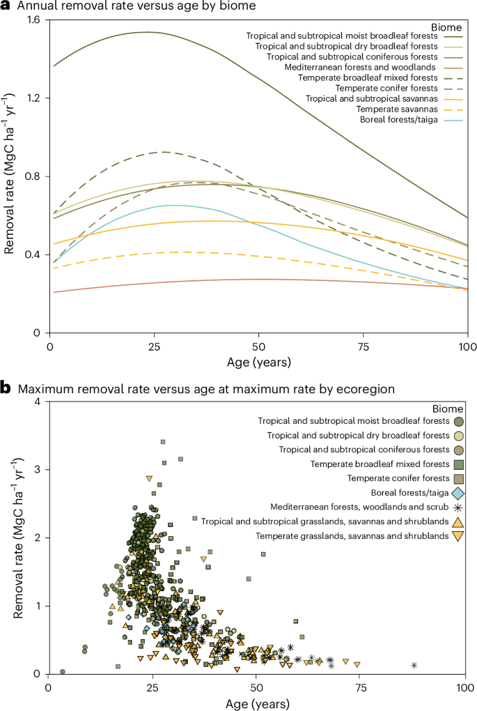
a, Annual carbon removal rates (MgC ha⁻¹ yr⁻¹) averaged by biome. b, Maximum carbon removal rate and age at which this occurrs (see also Fig. 2). Both panels show outputs from our model, with each point in b representing the modelled result for each individual ecoregion denoted with symbology for biome affiliation. Data are aggregated by biomes and ecoregions²² for visualization, but see Fig. 2 and Data availability for grid-level results.

We also examined the maximum carbon removal rate per grid (Figs. 1b and 2a) and found that it varies more than 200-fold across the globe (0.02–4.73 MgC ha⁻¹ yr⁻¹, mean 0.85 ± 0.54), typically peaking in 30 ± 12-year-old stands (Figs. 1b and 2b). The Mediterranean forests, woodland, and scrub biome²² has the lowest mean maximum rates (0.40 ± 0.33 MgC ha⁻¹ yr⁻¹, at 48 ± 19 years), while the tropical and subtropical moist broadleaf forest biome reaches the highest (1.57 ± 0.49 MgC ha⁻¹ yr⁻¹, at 23 ± 7 years). Most forested ecoregions²² (84%) attain maximum removal rates between 20 and 40 years (Fig. 1b) with some divergence. Central Polynesian tropical moist forests peak at 4 ± 4 years, while eastern Australian mulga shrublands peak at 74 ± 7 years. Overall, tropical moist forest ecoregions reach peak removals earliest (23 ± 7 years), followed by temperate broadleaf (25 ± 7 years) and savanna ecoregions later (Fig. 1b and Extended Data Fig. 3). Within tropical moist forests, regional differences in peak ages occur, which may reflect limited training data (lowering confidence) or could be indicative of actual ecological dynamics. Comparing maximum removal rates with their timing highlights where and how quickly substantial removals can be realized. Tropical/subtropical moist broadleaf forests and some temperate forests achieve high rates early, whereas boreal, Mediterranean and tropical/subtropical savanna ecoregions reach lower peaks later.

Fig. 2: Spatial distribution of the maximum growth rate achievable in 1–100-year-old secondary forests.

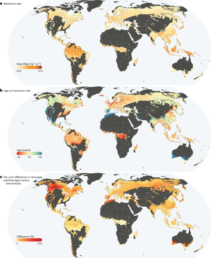
a, The maximum rate of annual carbon removal for each grid cell derived from the CR curves. b, The age at which this maximum rate occurs. c, The per cent difference in total removals over the optimal 25-year period versus new forests. Only forested biomes²² are shown. Maps created using QGIS version 3.34 with country boundaries from Natural Earth.

Capturing spatio-temporal variation in carbon removal rates improves estimates of natural forest regeneration’s mitigation potential within policy-relevant timeframes. For instance, if regeneration starts in 2025 across 800 Mha of identified reforestable area⁶, up to 20.3 billion MgC could be removed by 2050. Delaying until 2030 or 2035 reduces the potential to 15.9 or 11.6 billion MgC (22 and 43% lower, respectively). The disproportionate loses relative to their time delays emphasize the importance of swift action in initiating natural regeneration²³.

If the priority is maximizing per-hectare carbon removals from 2025 to 2050, existing secondary forests generally outperform new regeneration (Fig. 2c). The optimal 25-year window for each grid cell (19–43 years on average) could remove 20.7 ± 13.1 MgC ha⁻¹ on average, compared with 18.8 ± 12.4 MgC ha⁻¹ over the first 25 years of new regeneration. Although the average increase is 10%, some locations show gains of up to 820% during their optimal window compared with the first 25 years. Only 1.3% of grid cells achieve maximum removal rates during the earliest stages of regeneration.

We reserved 10,836 field estimates (~10%) for validation, independent from model training. Across all age classes, the model produced a root mean square error (RMSE) of 0.62 MgC ha⁻¹ yr⁻¹ and a coefficient of determination (R²) of 0.41. Error varied by age (Extended Data Fig. 4), with the 95-year class showing the lowest RMSE (0.30 MgC ha⁻¹ yr⁻¹) and the 90-year class the highest R² (0.58). The 5- and 10-year classes had the highest RMSE (1.93 MgC ha⁻¹ yr⁻¹) and lowest R² (0.22). Greater error in younger forests may stem from how starting carbon density was accounted for in the field data, as many stands begin with residual biomass, which probably varies by pre-regeneration land use, disturbance intensity or measurement protocols. The RMSE and R² generally stabilized beyond 20 years (Extended Data Fig. 4).

We also compared our curves with independent regional estimates (Amazon, Congo Basin and Borneo) derived from remote sensing and time-since-disturbance methods^19,20. Between the ages of 10 and 50 years, where growth rates typically peak (Fig. 3), our results aligned well. Discrepancies at younger ages may arise because Heinrich et al.^19,20 forced their curves to zero, whereas we let our model estimate the intercept to prevent rate over-estimation in the youngest stands (Fig. 3). Beyond 50 years, differences may reflect (1) the finite length of the Landsat archive (~40 years)²⁴; (2) biomass saturation in satellite-derived estimates²⁵; or (3) coarse spatial aggregation in remote sensing approaches. Our modelled rates also broadly match benchmark data for the Brazilian Amazon²⁶, which find ~80 MgC ha⁻¹ in 40-year-old stands. In comparison, our Amazon curves generally range between 50 and 100 MgC ha⁻¹ (Fig. 3a).

Fig. 3: Modelled aboveground carbon accumulation in three tropical regions (Amazon, Congo Basin and Borneo) compared with remote sensing-based estimates from refs. ^19,20.

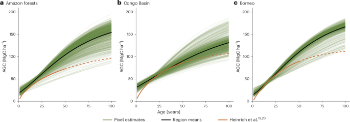
a–c, We used the same spatial boundaries as in Heinrich et al.^19,20, randomly sampled 1,000 grid cells from our dataset within each region (shown in green with black line indicating regional mean) and compared them with the remote sensing-derived curves (in orange). The dashed portion of the orange line indicates where the remote sensing curves have been extrapolated beyond available remote sensing imagery. We show results for three regions: Amazon forests (a), Congo Basin (b) and Borneo (c).

Compared with IPCC defaults¹⁷, our modelled rates are 26% lower in forests aged 20 years and under, and 18% higher in forests aged 21–100 years (Fig. 4). These differences vary by ecozone: in young forests, our rates vary from 44% lower (North America rainforest ecozone) to 81% higher (South America temperate mountain system ecozone), while in older forests, they range from 20% lower (North America mountain systems ecosystem ecozone) to 196% higher (South America subtropical mountain system ecozone). IPCC defaults fail to capture the 1.2- to 15.8-fold variation within ecozones, and they do not account for the rapid acceleration in young stands or slowing in older ones (Fig. 5). These findings underscore the need for regularly updated, high-resolution estimates rooted in the latest field data capture variable growth dynamics across space and time.

Fig. 4: Modelled carbon removal rates across global ecozones compared with IPCC default rates for young (≤20 years) and older (20–100 years) secondary forests.

a,b, Average predicted carbon removal rate per ecozone (yellow circles) compared with IPCC defaults (black circles) for older secondary forest (21–100 years; a) and young secondary forest (≤20 years; b). Yellow circles and coloured bars show the average carbon removal rate within the ecozone and range of grid cell values (5th–95th percentiles), respectively. Ecozone and continental forest types are indicated along the x axis. NA, North America; SA, South America.

Fig. 5: Modelled forest carbon removal rates by stand age in four ecozones, compared with IPCC defaults for young (≤20 years) and old (>20 years) secondary forests.

a–d, Rates of carbon removal by forest stands for four ecozones. Average rate through stand ages (solid green line) and the overall range across grid cells (5th–95th percentile; shaded area) are compared with IPCC default rates for young (≤20 years; orange dashed line) and old (>20 years; red dashed line) secondary forests. These ecozones show distinct patterns: IPCC defaults for young forests are higher (a); IPCC defaults align with model means but miss variability (b); IPCC defaults are generally higher (c); and IPCC defaults bracket our modelled values but miss substantial variability (d).

We produced global 1-km resolution AGC curves for 100 years of natural forest regeneration. Combined with maps of stand age and reforestable area, these curves enable estimates of carbon removals over policy-relevant timescales from any starting age. For instance, if 800 Mha of restorable forest area⁶ began regenerating in 2025, they could remove up to 20.3 billion MgC by 2050. Delaying by 5 or 10 years cuts that potential by roughly a quarter or a half, respectively. Established young secondary forests can provide more immediate and often greater per-hectare removals—up to 8-fold by 2050 (Fig. 2c). Delays in restoration²⁷, coupled with the lag before peak removal, further diminishes the mitigation potential of new regeneration.

Secondary forest as a vital natural climate solution

Preventing warming beyond Paris Agreement targets requires deploying all feasible mitigation strategies. While reducing fossil fuel emissions remains paramount, maintaining and increasing forest sinks is also vital^8,13. Young secondary forests warrant heightened attention as they can provide greater per-hectare carbon removals during critical climate and policy windows^12,28,29, and their potential for removals is more assured than new regeneration, which may fail under unfavourable starting conditions. For instance, seed sources or dispersers may be absent, or rising temperatures may constrain germination^30,31,32,33. Protecting at-risk secondary forests provides the climate mitigation benefits of both securing on-going peak removals and avoiding release of in situ carbon stocks³⁴.

Climate mitigation through forest protection often focuses on intact and mature forests, given their high in situ carbon and biodiversity value^35,36, which remains a crucial strategy³⁷. Young forests, however, face escalating threats. Across Latin America, secondary forest loss is ten times more likely than persistence³⁸. In the Brazilian Amazon, half of secondary forests are cleared within 8 years of establishment³⁹, while in wet Costa Rican forests, the average age at clearance is 20 years⁴⁰. Our estimates show that 8-year-old forest in the Brazilian Amazon would remove 36% more carbon from the atmosphere by 2030 than newly growing stands (7.7 versus 10.5 MgC ha⁻¹ from 2025 to 2030). Similarly, a 20-year-old wet Costa Rican forest would remove 65% more (7.9 versus 13.0 MgC ha⁻¹). Thus, prioritizing protection of at-risk young secondary forests for rapid carbon removal, alongside at-risk older stands with large carbon stocks, represents a crucial climate mitigation action.

However, there are limited mechanisms to protect young secondary forests. No carbon market methodologies currently credit protecting or improving management in very young secondary forests²⁹. Rules require at least 10 years of cleared land prior to reforestation projects, while forest protection projects require forests to be at least 10 years old. Improved forest management projects only apply in places with logging operations, covering a fraction of secondary forests²⁹.

For natural forest regeneration to be recognized as a climate mitigation action, several criteria must be met^41,42. First, additionality—the forest must be at risk of conversion or unlikely to grow under current conditions. This can be difficult to demonstrate for existing forests³⁷, although newer dynamic baseline approaches enable comparing project areas to non-project areas to better estimate additionality. Second, durability, meaning the carbon must remain stored for decades to centuries⁴¹. Our model is built on empirical data inclusive of background mortality rates, because individual trees that die are excluded from the measurement of aboveground live carbon. This makes the estimate somewhat conservative in that it ignores carbon storage within dead pools. However, it does not account for potential increases in disturbance and mortality with future climate change⁴³. Partial or stand-clearing disturbances would release some to all of the carbon back to the atmosphere, and these larger disturbances are not integrated into our growth curves.

Although we estimate up to 20.3 billion MgC could be removed by 2050 across 800 Mha, a full global potential assessment requires data on forest age, in situ carbon and future disturbance risk. Existing global forest age and biomass maps^44,45 do not clearly distinguish regeneration from production forests⁴⁶, nor predict future changes in forest cover⁴⁷. Nevertheless, our analysis shows that on a per-hectare basis, protecting at-risk secondary forests over their peak removal window can deliver about 10% greater removal rates on average—and up to 820% more in some locations—compared with initiating new regeneration (Fig. 2c). Alongside designating new areas of land for regeneration, these findings highlight the value of protecting existing secondary forests, and potentially implementing management that removes impediments to natural regeneration (for example, invasive liana removals).

Caveats and future directions

Despite the insights gained, several caveats highlight avenues for deeper investigation. First, the socio-economic context of forest regeneration and the role of local communities must be recognized and prioritized^48,49. Many secondary forests, as well as lands targeted for regeneration, are used by low-income, rural communities for livelihoods such as those based in shifting cultivation. Climate finance must account for detrimental effects on livelihoods, as natural climate solutions should not come at the expense of human rights and local development⁴¹. Engaging local communities and integrating their needs and knowledge into forest management is vital for achieving multiple sustainable and equitable outcomes. Trade-offs often arise among biodiversity, ecosystem service provisions and rural employment, and prioritization across multiple outcomes can highlight solutions that optimize the multiple benefits desired from restoration of forest cover and forest protection^50,51.

Second, although our data include savanna and grassland biomes, they show limited and slow carbon removal (Fig. 1), aligning with evidence that tree establishment in savannas offers limited mitigation potential⁵². Frequent fire disturbance may also prevent stands from reaching ages of rapid removal⁵³. These biomes have distinct biodiversity and carbon cycling processes. Their management for climate mitigation may demand tailored and nuanced approaches apart from forest regeneration^54,55. Hence, caution is warranted when considering forest-focused climate mitigation strategies in non-forested systems.

Third, our plot data are heavily biased towards northern temperate forests (Extended Data Figs. 5 and 6). Improving field data coverage in underrepresented regions would increase confidence in our predictions. Integrating field and remoting sensing data would help to both fill spatial gaps in the field data and temporal gaps in the remote sensing data.

Fourth, additional steps could enhance both the completeness and accuracy of our carbon removal estimates. We focused on AGC, but incorporating other pools (for example, soil carbon) would provide more comprehensive results. Our projections are based on average historical climate, with their application across longer time horizons limited. Future work should incorporate climate change impacts on removal rates and the durability of stored carbon⁵⁶. We also did not assess the initial disturbance type of the plots, which may influence establishment, initial biomass and subsequent removal rates. Factors like site degradation¹⁹, fine-scale environmental variation (for example, slope, proximity to roads)⁵⁷ and presence of seed dispersal³³ further impact the likelihood of regeneration and pace of carbon removal. However, our data can be combined with maps of the likelihood of natural regeneration to further refine estimates of mitigation potential⁵⁸. Finally, inconsistencies with how the stand ages were calculated and reported in the inventory data (for example, even- versus uneven-aged stands) may introduce noise into our results. Local analyses remain critical to refine these estimates for specific sites or projects.

Overview

To create global maps of carbon removal rates in naturally regenerating forests, we merged field measurements of carbon stocks at known stand ages with an extensive set of environmental factors known to affect carbon densities and removal rates. We then predicted carbon densities in 5-year age intervals from 5 to 100 years using multiple random forest models at a spatial resolution of approximately 1 km for the global terrestrial surface. Finally, we fitted a CR growth curve to each carbon density grid cell to create global maps of the CR curve parameters (Extended Data Fig. 1).

Assembling a global dataset of AGC field measurements

We assembled a global dataset of age-specific AGC estimates from field measurements in naturally regenerating forest areas, combining national and provincial forest inventory data with literature-extracted data.

We examined forest inventory data from Australia (2006–2017, N = 58), Canada (1926–2018, N = 52,737), the Netherlands (2001–2020, N = 3,577), Sweden (2007–2017, N = 26,805) and the USA (1999–2020, N = 135,289). Selection criteria required plots to be in naturally regenerating stands with documented age, geolocation and aboveground biomass or carbon measurements expressible in Mg ha⁻¹. For inventory data from Quebec, aboveground biomass was calculated from tree-level data in 5,191 permanent sample plots with information about tree species, age and diameter at breast height. To convert from diameter at breast height to biomass, we used allometric equations from the Canadian national biomass equations^60,61 and then aggregated tree-level data to the plot level. Finally, we noted that many forest inventory datasets adjusted plot geolocations by ~1 km to adhere to security protocols; this aggregation aligned with our spatial resolution.

Our literature-derived data, sourced from a systematic review of 11,360 studies by Cook-Patton et al.⁸, supplemented the inventory data and expanded its geographic coverage. Following the methods in Cook-Patton et al.⁸, we reviewed 330 additional recent studies (that is, published between 19 April 2017 and 13 August 2021), maintaining the same selection criteria focused on empirical measures of AGC, stand age and geolocation for naturally regenerating forest plots.

To ensure consistency and accuracy, we standardized data across sources, excluding duplicates, erroneous locations (for example, locations within water bodies), stands younger than one year and outliers (AGC ± 3 s.d. from the mean for each age). The refined dataset comprised 172,585 AGC measurements, temporally and spatially aggregated into 20 age class bins, corresponding to 5-year intervals centred on 5, 10, 15,…90, 95, 100 years. For each age class, we computed the mean AGC within ~1-km grid cells, using cell centroids for geolocation, culminating in 109,708 estimates of AGC (Extended Data Fig. 5).

Modelling AGC densities for 0–100-year-old forests

We estimated AGC densities in naturally regenerating forests aged up to 100 years, by using a spatial predictive model combining the global dataset of field-based estimates with 66 environmental covariates, as developed by Cook-Patton et al.⁸. The covariates encompassed a range of factors including climate, soil nutrients, chemical and physical properties, radiation, topography and nitrogen deposition, in addition to a categorical biome variable (Extended Data Table 2), and reflected long-term average conditions since 1970. The covariates were standardized on a WGS84 grid at 30 arcsec (~1 km² at the Equator.) We downsampled higher-resolution data using mean aggregation and applied direct sampling without interpolation for upsampling lower-resolution data.

Following the approach in Cook-Patton et al.⁸, we employed random forest models using all environmental variables. We reserved approximately 10% of our data for validation (10,836 points), and excluded these from the model training process that utilized the remaining 98,872 points. The validation data were selected randomly within each age class. However, to reduce effects of spatial autocorrelation, points were not used for validation if they were within 10 km of any training data. The underlying field data, all from naturally regenerating forests, spanned 50 countries, with a strong concentration in temperate regions such as Canada, the USA and Europe (Extended Data Fig. 5), with a slight concentration in older age classes (~60–80 years; Extended Data Fig. 6). Despite some geographic gaps, particularly in tropical forest biomes (Extended Data Table 1), our dataset marked a substantial enhancement from previous efforts⁸, with improved geographic coverage in Canada, Europe, China, Russia and South America.

We constructed a unique model to estimate AGC density for each forest age class rather than a single model for across all age classes. To tune the model parameters, we applied three-fold cross-validation. Data for each age class were segmented into three equal parts: two were combined for training and the third served as a validation set. We assessed model performance through three rounds of validation, each time rotating the validation subset, and selecting hyper-parameters based on the lowest average RMSE from the tree iterations.

We implemented a Monte Carlo approach to develop an ensemble model for our initial AGC density model predictions and uncertainty for each age class. We developed the ensemble model by bootstrapping 100 independent samples (randomly selected 80% of the training data with replacement) for each age class. We then trained individual random forest models on each of the 100 samples using the optimized set of hyper-parameters, resulting in 100 predictions of AGC density for each grid cell for each age class. From these estimates, we quantified cell-level model uncertainty by calculating the standard deviation and error ratio among the ensemble predictions for each age class (see Data availability). The modelling process to this point, including machine learning operations, was conducted in Google Earth Engine⁶².

CR curve calculation

Our random forest models generated global maps of carbon densities for forest age classes. We then fitted the CR growth function through the 5-year estimates of AGC density at each cell. We did this for two reasons. First, carbon density in each age class is dependent on carbon density in proceeding age classes. Second, because our plot data are not consistently distributed across space and age classes, the initial model outputs sometimes show erratic or declining carbon densities between sequential age classes, as highlighted in Extended Data Fig. 7. A CR growth function thus helps to smooth out age-based variation and more accurately mirror the natural progression of forest maturation.

The CR function, a staple in forest growth modelling⁶³, provides a versatile framework capable of encapsulating either sigmoidal or logarithmic growth trajectories. It is expressed through the formula:

where y denotes the accumulated carbon at time t; A represents the asymptotic carbon accumulation limit; b impacts the initial carbon density; m is a shape-controlling parameter; k signifies the growth rate; and e is the base of the natural logarithm. For this study, we set m at 0.67 (ref. ²¹). We optimized and produced 1-km-resolution maps of A, b and k based on our dataset. While many approaches assume initial carbon density to be 0 at stand initiation^16,19, we optimized this parameter. Our model often predicted at least some AGC density at stand initiation (that is, b < 1.0; Extended Data Fig. 2c), except at some northern latitudes where stand-clearing disturbances (for example, wildfire and clearcut harvest) are common⁶⁴. This reduced error may reflect realistic conditions where some residual biomass remains at stand initiation and leads to more conservative estimates of carbon removal rates at the youngest stand ages.

We utilized the nonlinear least squares method in R from the base STATS package to optimize the A, b and k parameters of the CR model for each cell, using the AGC density estimates from our random forest models. The optimization leveraged 100 AGC density estimates per cell per age class from the random forest ensemble. We exported global data for each age class from Google Earth Engine in 5° tiles, resulting in twenty 100-band images per tile. We also exported potential maximum carbon density values, calculated as the maximum of our estimates or those from Walker et al.⁶⁵, as starting values for A in the optimization.

In R, we loaded all images for a tile and converted them into a single vector of cell values, along with vectors of corresponding age values and potential maximum density. For each cell, relevant values were extracted, and the nonlinear least squares optimization was performed. Starting values were set for each parameter (A—maximum potential from ref. ⁶⁵, k—0.5 and b—0.75). A was allowed to vary up to 10% of the starting value, k between 0.01 and 0.1, and b between 0.2 and 1. If non-convergence occurred for a grid cell, updated estimates were set as new starting values, and the optimization was repeated, up to four times, ensuring convergence for all cells. The resulting parameters and standard errors were stored and converted back to raster datasets with the same resolution and grid as the original data.

We employed parallel processing capabilities in R using the doParallel (v. 1.0.17) package, which enabled simultaneous processing of individual tiles across available computer cores, substantially improving computation time.

This approach enabled us to generate refined global maps with ~1-km resolution. Fitting CR curves through the 5-year carbon density estimates at each grid cell smoothed out the fluctuations and resulted in detailed maps of the CR curve parameters: the asymptote (A; Extended Data Fig. 2a) represented the maximum potential carbon density (MgC ha⁻¹), the growth rate coefficient (k; Extended Data Fig. 2b) and the initial carbon density coefficient (b; Extended Data Fig. 2c) at time zero. Globally, maximum potential carbon density (A) ranged from 27 to 187 MgC ha⁻¹ (5th–95th percentile), with the greatest values generally in carbon-dense, moist tropical forests and lowest in boreal forests (Extended Data Fig. 2a). Higher k values led to steeper CR curves, and we found that the highest k values concentrated in northern latitudes and moist tropical forests, whereas savannas have lower k values, suggesting that it takes longer to achieve the maximum carbon removal in these drier ecosystems (Extended Data Fig. 2b). Combining the cell-level parameter with an assumed default for the remaining parameter (m) made it possible to construct grid-level growth curves that predict changes in AGC storage (MgC ha⁻¹) through time.

Validation and comparisons

From our growth curves we extracted the total AGC density corresponding to the locations and age classes for each point from our reserved validation dataset (n = 10,836). With these data we calculated the RMSE and R². We calculated these for all results pooled as well as each age class independently.

We compared the growth curves generated by our model with those derived independently through remote sensing^19,20. These studies combined estimates of time since disturbance (that is, forest age) with biomass maps across three large geographical regions: the Congo Basin, Amazon Basin and Borneo forests. Within the spatial extents as used by Heinrich et al.¹⁹ for each region, we extracted the growth curves for 1,000 random points as well as the mean growth curve across all cells. We plotted these curves along with the regional curves for each region as developed by Heinrich et al.¹⁹.

Comparison to IPCC

We compared our predicted rates with the latest IPCC default rates for both young (≤20-year-old) and old (21–100-year-old) secondary forests. For each cell, we estimated the rate of carbon removal for young and old forests, by averaging the annual removal rates for each of each of the age classes. We then aggregated these, calculating the minimum, maximum and mean, across each ecozone–continent combination (Fig. 4). Note that the IPCC defaults were calculated by dividing predicted carbon density (MgC ha⁻¹) by stand age¹⁶. This led to inflated estimates of carbon removal if the stand contained residual biomass. Thus, we did not mimic these methods, but instead used our more conservative estimates based on changes in AGC.

Reporting summary

Further information on research design is available in the Nature Portfolio Reporting Summary linked to this article.

Data outputs for the CR growth curve parameters (A, k, b), along with their standard error and the global maps used in Fig. 2, are available via Zenodo at https://doi.org/10.5281/zenodo.15090826 (ref. ⁶⁶). The data can also be visualized and explored via a web application at https://ee-groa-carbon-accumulation.projects.earthengine.app/view/natural-forest-regeneration-carbon-accumulation-explorer. Source data for reproducing the figures and analyses are available via GitHub at https://github.com/naturalclimatesolutions/nat_for_regen_c_accumulation or via Zenodo at https://doi.org/10.5281/zenodo.15078013 (ref. ⁶⁷). Plot data from Alberta, British Columbia, Saskatchewan and the Netherlands were collected and harmonized by T.A.M.P. and A.E.-M., but accessed via data-sharing agreements with the original institutions (Alberta: https://www.alberta.ca/permanent-sample-plots-program; British Columbia: https://www2.gov.bc.ca/gov/content/industry/forestry/managing-our-forest-resources/forest-inventory/ground-sample-inventories; Saskatchewan: https://geohub.saskatchewan.ca/; and the Netherlands: https://doi.org/10.1007/s10342-014-0781-y). Data for Quebec were collected and harmonized by C.R.D. and accessed via agreements with the original institution (https://www.donneesquebec.ca/recherche/dataset/placettes-echantillons-permanentes-1970-a-aujourd-hui). Inventory data for Sweden and Australia were collected and harmonized by D.A.G. and can be accessed via the original institutions (Sweden: https://www.slu.se/en/Collaborative-Centres-and-Projects/the-swedish-national-forest-inventory/; Australia: https://doi.org/10.1016/j.foreco.2019.117838 (ref. ⁶⁸). The United States inventory data were acquired the USDA FIA programme (https://research.fs.usda.gov/programs/fia). The literature-derived dataset is available via Zenodo at https://doi.org/10.5281/zenodo.15078013 (ref. ⁶⁷). Owing to data size limitations, we provide a subset of the data (northwest USA) in the GitHub repository. Subsets of data for other locations can be provided by the corresponding author (N.R.) on request ([email protected]).

References

Authors and Affiliations

1. The Nature Conservancy, Worthington, MA, USA

   Nathaniel Robinson

2. CIFOR-ICRAF, Nairobi, Kenya

   Nathaniel Robinson

3. Nature United, Toronto, Ontario, Canada

   C. Ronnie Drever

4. World Resources Institute, Washington, DC, USA

   David A. Gibbs & Kristine Lister

5. Nicholas School of the Environment Master of Environmental Management Program, Duke University, Durham, NC, USA

   Kristine Lister

6. School of Geography, Earth and Environmental Sciences, University of Birmingham, Birmingham, UK

   Adriane Esquivel-Muelbert & Thomas A. M. Pugh

7. Birmingham Institute of Forest Research, University of Birmingham, Birmingham, UK

   Adriane Esquivel-Muelbert & Thomas A. M. Pugh

8. Remote Sensing and Geoinformatics Division, Helmholtz Centre for GeoSciences (GFZ), Potsdam, Germany

   Viola Heinrich

9. School of Geographical Sciences, University of Bristol, Bristol, UK

   Viola Heinrich

10. Laboratoire des Sciences du Climat et de l’Environnement, Université Paris-Saclay, Gif sur Yvette, France

    Philippe Ciais & Yidi Xu

11. Instituto de Pesquisa Ambiental da Amazônia - IPAM, Brasília, Brazil

    Celso H. L. Silva-Junior

12. Programa de Pós-Graduação em Biodiversidade e Conservação, Universidade Federal do Maranhão (UFMA), São Luís, Brazil

    Celso H. L. Silva-Junior

13. CTrees, Pasadena, CA, USA

    Zhihua Liu & Sassan Saatchi

14. Department of Physical Geography and Ecosystem Science, Lund University, Lund, Sweden

    Thomas A. M. Pugh

15. NASA Jet Propulsion Laboratory, Pasadena, CA, USA

    Sassan Saatchi

16. The Nature Conservancy, Arlington, VA, USA

    Susan C. Cook-Patton

17. Smithsonian Environmental Research Center, Edgewater, MD, USA

    Susan C. Cook-Patton

Contributions

N.R., A.E.-M., D.A.G., S.C.C.-P., T.A.M.P. and C.R.D. compiled national inventory data. N.R., K.T., S.C.C.-P. and V.H. compiled literature-derived data. N.R. and K.L. constructed the spatial models. N.R. conducted all the analyses. N.R. and S.C.C.-P. wrote the manuscript. All authors discussed the results and contributed to the writing and review of the paper.

Corresponding authors

Correspondence to Nathaniel Robinson or Susan C. Cook-Patton.

Competing interests

The authors declare no competing interests.

Peer review information

Nature Climate Change thanks Robin Chazdon and the other, anonymous, reviewer(s) for their contribution to the peer review of this work.

Open Access This article is licensed under a Creative Commons Attribution 4.0 International License, which permits use, sharing, adaptation, distribution and reproduction in any medium or format, as long as you give appropriate credit to the original author(s) and the source, provide a link to the Creative Commons licence, and indicate if changes were made. The images or other third party material in this article are included in the article’s Creative Commons licence, unless indicated otherwise in a credit line to the material. If material is not included in the article’s Creative Commons licence and your intended use is not permitted by statutory regulation or exceeds the permitted use, you will need to obtain permission directly from the copyright holder. To view a copy of this licence, visit http://creativecommons.org/licenses/by/4.0/.

Reprints and permissions

References

Callaghan, M. et al. Machine-learning-based evidence and attribution mapping of 100,000 climate impact studies. Nat. Clim. Change 11, 966–972 (2021).
Forster, P. M. et al. Indicators of global climate change 2022: annual update of large-scale indicators of the state of the climate system and human influence. Earth Syst. Sci. Data 15, 2295–2327 (2023).
IPCC Climate Change 2022: Mitigation of Climate Change (eds Shukla, P. R. et al.) (Cambridge Univ. Press, 2022).
Fuss, S. et al. Negative emissions—part 2: costs, potentials and side effects. Environ. Res. Lett. 13, 063002 (2018).
Young, J. et al. The cost of direct air capture and storage can be reduced via strategic deployment but is unlikely to fall below stated cost targets. One Earth 6, 899–917 (2023).
Griscom, B. W. et al. Natural climate solutions. Proc. Natl Acad. Sci. USA 114, 11645–11650 (2017).
Roe, S. et al. Contribution of the land sector to a 1.5 °C world. Nat. Clim. Change 9, 817–828 (2019).
Cook-Patton, S. C. et al. Mapping carbon accumulation potential from global natural forest regrowth. Nature 585, 545–550 (2020).
Drever, C. R. et al. Natural climate solutions for Canada. Sci. Adv. 7, eabd6034 (2021).
Lewis, S. L., Wheeler, C. E., Mitchard, E. T. A. & Koch, A. Restoring natural forests is the best way to remove atmospheric carbon. Nature 568, 25–28 (2019).
Fargione, J. et al. Challenges to the reforestation pipeline in the United States. Front. Glob. Change 4, 629198 (2021).
Busch, J. et al. Cost-effectiveness of natural forest regeneration vs. plantations for climate mitigation. Nat. Clim. Change 14, 996–1002 (2024).
Chazdon, R. L. & Guariguata, M. R. Natural regeneration as a tool for large‐scale forest restoration in the tropics: prospects and challenges. Biotropica 48, 716–730 (2016).
Gilroy, J. J. et al. Cheap carbon and biodiversity co-benefits from forest regeneration in a hotspot of endemism. Nat. Clim. Change 4, 503–507 (2014).
Crouzeilles, R. et al. Achieving cost‐effective landscape‐scale forest restoration through targeted natural regeneration. Conserv. Lett. 13, e02448 (2020).
Suarez, D. R. et al. Estimating aboveground net biomass change for tropical and subtropical forests: refinement of IPCC default rates using forest plot data. Glob. Change Biol. 25, 3609–3624 (2019).
Nabuurs, G.-J. et al. in Climate Change 2022: Mitigation of Climate Change (eds Shukla, P. R. et al.) Ch. 7 (IPCC, Cambridge Univ. Press, 2022).
Chen, X., Luo, M. & Larjavaara, M. Effects of climate and plant functional types on forest above-ground biomass accumulation. Carbon Balance Manag. 18, 5 (2023).
Heinrich, V. H. A. et al. The carbon sink of secondary and degraded humid tropical forests. Nature 615, 436–442 (2023).
Heinrich, V. H. A. et al. Large carbon sink potential of secondary forests in the Brazilian Amazon to mitigate climate change. Nat. Commun. 12, 1785 (2021).
Bukoski, J. J. et al. Rates and drivers of aboveground carbon accumulation in global monoculture plantation forests. Nat. Commun. 13, 4206 (2022).
Dinerstein, E. et al. An ecoregion-based approach to protecting half the terrestrial realm. Bioscience 67, 534–545 (2017).
Qin, Z. et al. Delayed impact of natural climate solutions. Glob. Change Biol. 27, 215–217 (2021).
Vancutsem, C. et al. Long-term (1990–2019) monitoring of forest cover changes in the humid tropics. Sci. Adv. 7, eabe1603 (2021).
Araza, A. et al. A comprehensive framework for assessing the accuracy and uncertainty of global above-ground biomass maps. Remote Sens. Environ. 272, 112917 (2022).
Giles, A. L. et al. Simple ecological indicators benchmark regeneration success of Amazonian forests. Commun. Earth Environ. 5, 780 (2024).
Forests Under Fire: Tracking Progress on 2030 Forest Goals (Forest Declaration Assessment, 2024); https://forestdeclaration.org/wp-content/uploads/2024/10/2024ForestDeclarationAssessment.pdf
Moomaw, W. R., Masino, S. A. & Faison, E. K. Intact forests in the United States: proforestation mitigates climate change and serves the greatest good. Front. Glob. Change 2, 27 (2019).
Brancalion, P. H. S. et al. A call to develop carbon credits for second-growth forests. Nat. Ecol. Evol. 8, 179–180 (2024).
Chazdon, R. L. Landscape restoration, natural regeneration, and the forests of the future. Ann. Missouri Bot. Gard. 102, 251–257 (2017).
Crouzeilles, R. et al. A new approach to map landscape variation in forest restoration success in tropical and temperate forest biomes. J. Appl. Ecol. 56, 2675–2686 (2019).
Holden, Z. A. et al. Low-elevation forest extent in the western United States constrained by soil surface temperatures. Nat. Geosci. 17, 1249–1253 (2024).
Bello, C. et al. Frugivores enhance potential carbon recovery in fragmented landscapes. Nat. Clim. Change 14, 636–643 (2024).
Mo, L. et al. Integrated global assessment of the natural forest carbon potential. Nature 624, 92–101 (2023).
Noon, M. L. et al. Mapping the irrecoverable carbon in Earth’s ecosystems. Nat. Sustain 5, 37–46 (2022).
Watson, J. E. M. et al. The exceptional value of intact forest ecosystems. Nat. Ecol. Evol. 2, 599–610 (2018).
Cook-Patton, S. C. et al. Protect, manage and then restore lands for climate mitigation. Nat. Clim. Change 11, 1027–1034 (2021).
Schwartz, N. B., Aide, T. M., Graesser, J., Grau, H. R. & Uriarte, M. Reversals of reforestation across Latin America limit climate mitigation potential of tropical forests. Front. Glob. Change 3, 85 (2020).
Nunes, S., Oliveira, L., Siqueira, J., Morton, D. C. & Souza, C. M. Unmasking secondary vegetation dynamics in the Brazilian Amazon. Environ. Res. Lett. 15, 034057 (2020).
Reid, J. L., Fagan, M. E., Lucas, J., Slaughter, J. & Zahawi, R. A. The ephemerality of secondary forests in southern Costa Rica. Conserv. Lett. 12, e12607 (2019).
Ellis, P. W. et al. The principles of natural climate solutions. Nat. Commun. 15, 547 (2024).
VM0047 (2025) Afforestation, Reforestation, and Revegetation Version 1.1 Sectoral Scope 14: Agriculture, forestry and other land use (AFOLU), VCS. https://verra.org/methodologies/vm0047-afforestation-reforestation-and-revegetation-v1-1/
Anderegg, W. R. L. et al. A climate risk analysis of Earth’s forests in the 21st century. Science 377, 1099–1103 (2022).
Besnard, S. et al. Mapping global forest age from forest inventories, biomass and climate data. Earth Syst. Sci. Data 13, 4881–4896 (2021).
Santoro, M. & Cartus, O. ESA Biomass Climate Change Initiative (Biomass_cci): Global Datasets of Forest Above-ground Biomass for the Years 2010, 2017, 2018, 2019 and 2020, V4. CEDA Archivehttps://doi.org/10.5285/af60720c1e404a9e9d2c145d2b2ead4e (2021).
Pugh, T. A. M., Arneth, A., Kautz, M., Poulter, B. & Smith, B. Important role of forest disturbances in the global biomass turnover and carbon sinks. Nat. Geosci. 12, 730–735 (2019).
Nölte, A., Yousefpour, R., Cifuentes-Jara, M. & Hanewinkel, M. Sharp decline in future productivity of tropical reforestation above 29 °C mean annual temperature. Sci. Adv. 9, eadg9175 (2023).
Fleischman, F. et al. Pitfalls of tree planting show why we need people-centered natural climate solutions. Bioscience 70, 947–950 (2020).
Shyamsundar, P. et al. Scaling smallholder tree cover restoration across the tropics. Glob. Environ. Change 76, 102591 (2022).
Drever, C. R. et al. Synergies and trade-offs for restoration of forest cover in Canada. One Earth 8, 101177 (2025).
Strassburg, B. B. N. et al. Strategic approaches to restoring ecosystems can triple conservation gains and halve costs. Nat. Ecol. Evol. 3, 62–70 (2019).
Hasler, N. et al. Accounting for albedo change to identify climate-positive tree cover restoration. Nat. Commun. 15, 2275 (2024).
Hoffmann, W. A. et al. Ecological thresholds at the savanna–forest boundary: how plant traits, resources and fire govern the distribution of tropical biomes. Ecol. Lett. 15, 759–768 (2012).
Veldman, J. W. et al. Tyranny of trees in grassy biomes. Science 347, 484–485 (2015).
Zhou, Y. et al. Limited increases in savanna carbon stocks over decades of fire suppression. Nature 603, 445–449 (2022).
Liu, Y. Y. et al. Recent reversal in loss of global terrestrial biomass. Nat. Clim. Change 5, 470–474 (2015).
Teixeira, A. M. G., Soares-Filho, B. S., Freitas, S. R. & Metzger, J. P. Modeling landscape dynamics in an Atlantic rainforest region: implications for conservation. For. Ecol. Manag. 257, 1219–1230 (2009).
Williams, B. et al. The global potential for natural regeneration in deforested tropical regions. Nature 636, 131–137 (2024).
Sewell, A., van der Esch, S. & Löwenhardt, H. Goals and Commitments for the Restoration Decade: A Global Overview of Countries’ Restoration Commitments Under the Rio Conventions and Other Pledges (PBL Netherlands Environmental Assessment Agency, 2020); https://www.pbl.nl/sites/default/files/downloads/pbl-2020-goals-and-commitments-for-the-restoration-decade-3906.pdf
Ung, C.-H., Bernier, P. & Guo, X.-J. Canadian national biomass equations: new parameter estimates that include British Columbia data. Can. J. For. Res. 38, 1123–1132 (2008).
Lambert, M.-C., Ung, C.-H. & Raulier, F. Canadian national tree aboveground biomass equations. Can. J. For. Res. 35, 1996–2018 (2005).
Gorelick, N. et al. Google Earth Engine: planetary-scale geospatial analysis for everyone. Remote Sens. Environ. 202, 18–27 (2017).
Pienaar, L. V. & Turnbull, K. J. The Chapman–Richards generalization of von Bertalanffy’s growth model for basal area growth and yield in even-aged stands. For. Sci. 19, 2–22 (1973).
Gauthier, S., Bernier, P., Kuuluvainen, T., Shvidenko, A. Z. & Schepaschenko, D. G. Boreal forest health and global change. Science 349, 819–822 (2015).
Walker, W. S. et al. The global potential for increased storage of carbon on land. Proc. Natl Acad. Sci. USA 119, e2111312119 (2022).
Robinson, N. et al. Data outputs for: Protect young secondary forests for optimum carbon removal. Zenodo https://doi.org/10.5281/zenodo.15090826 (2025).
Robinson, N. et al. naturalclimatesolutions/nat_for_regen_c_accumulation: Code for the publication: Protect young secondary forests for optimum carbon removal. Zenodo https://doi.org/10.5281/zenodo.15078013 (2025).
Paul, K. I. & Roxburgh, S. H. Predicting carbon sequestration of woody biomass following land restoration. For. Ecol. Manag. 460, 117838 (2020).
Trabucco, A. & Zomer, R. Global aridity index and potential evapotranspiration (ET0) climate database v2. Figshare https://doi.org/10.6084/m9.figshare.7504448.v3 (2019).
Hengl, T. et al. SoilGrids250m: global gridded soil information based on machine learning. PLoS ONE. 12, e016978 (2017).
Kriticos, D. J. et al. CliMond: global high resolution historical and future scenario climate surfaces for bioclimatic modelling. Methods Ecol. Evol. 3, 53–64 (2012).
Danielson, J. J. & Gesch, D. B. Global Multi-Resolution Terrain Elevation Data 2010 (GMTED2010). US Geological Survey (2011) https://pubs.usgs.gov/of/2011/1073/pdf/of2011-1073.pdf
Lamarque, J.-F. et al. Historical (1850–2000) gridded anthropogenic and biomass burning emissions of reactive gases and aerosols: methodology and application. Atmos. Chem. Phys. 10, 7017–7039 (2010).
Karlsson, K.-G. et al. CLARA-A2: CM SAF Cloud, Albedo and Surface Radiation Dataset from AVHRR Data - Edition 2 (CM SAF, 2017); https://wui.cmsaf.eu/safira/action/viewDoiDetails?acronym=CLARA_AVHRR_V002
Abatzoglou, J. T., Dobrowski, S. Z., Parks, S. A. & Hegewisch, K. C. TerraClimate, a high-resolution global dataset of monthly climate and climatic water balance from 1958–2015. Sci Data 5, 170191 (2018).
Fick, S. E. & Hijmans, R. J. WorldClim 2: new 1‐km spatial resolution climate surfaces for global land areas. Int. J. Climatol. 37, 4302–4315 (2017).
Acknowledgements
This work was primarily supported by the Bezos Earth Fund. C.H.L.S.-J. was supported by funding from the National Council for Scientific and Technological Development (CNPq) under the project YBYRÁ-BR: Space-Time Quantification of CO2 Emissions and Removals by Brazilian Forests (CNPq Process 401741/2023-0). T.A.M.P. and A.E.-M. were supported by funding from the European Research Council (ERC) under the European Union’s Horizon 2020 research and innovation programme (grant agreement no. 758873, TreeMort). This study is a contribution to the Swedish Research Council’s strategic research areas BECC and MERGE and the Nature-based Future Solutions profile area at Lund University. V.H. was supported by the CGIAR MITIGATE+ project, the WRI Land and Carbon Lab, and the Open EarthMonitor Project funded by the European Union (grant agreement no.101059548).
Ethics declarations