.png)

We are excited to announce that Redis Query Engine now supports Quantization and Dimensionality Reduction for vector search. This is based on an Intel and Redis partnership leveraging Intel SVS-VAMANA with multiple compression strategies.
Redis has always been the go-to choice for agents and applications demanding blazing-fast performance, and our community knows this comes with a direct relationship: memory usage equals operational cost. As vector search has become increasingly popular for powering AI applications, from recommendation engines to powering specialized agents, we've consistently heard from developers and operations teams about a common challenge: the memory footprint of high-dimensional embeddings can quickly become a budget concern.
Here's the reality: when you're running vector search workloads on Redis, every vector stored in memory directly impacts your infrastructure costs. A typical deployment with millions of 768-dimensional vectors (common with modern embedding models) can consume hundreds of gigabytes of RAM. For organizations scaling their AI applications, this memory requirement often becomes the primary cost driver.
But what if you could dramatically reduce that memory footprint without sacrificing the search quality and performance that made you choose Redis in the first place? With a comprehensive compression strategy - Quantization and Dimensionality Reduction, we can reduce the total memory footprint by 26–37%, while preserving search quality and performance.
Dive into the compression technology
Modern vector similarity search faces a fundamental challenge: as datasets scale to billions of vectors with hundreds or thousands of dimensions, memory footprint becomes the dominant deployment constraint and memory bandwidth emerges as a primary performance bottleneck. Traditional approaches to million-scale similarity search have struggled with the dual pressure of maintaining search accuracy while managing memory footprint, particularly when dealing with the random memory access patterns inherent in graph-based algorithms.
For context, storing 100 million vectors with 1536 dimensions in single-precision floating-point format requires 572GB of memory. This scale makes traditional exact nearest vector search (like using FLAT index in Redis) impractical, necessitating approximate methods that can operate within reasonable memory constraints while maintaining acceptable accuracy levels.
Intel SVS-VAMANA foundations
SVS-VAMANA combines the Vamana graph-based search algorithm, introduced by Subramanya et al., with Intel’s compression technology: LVQ and LeanVec.
Vamana is similar to HNSW in its use of proximity graphs for efficient search. Unlike HNSW’s multi-layered structure, Vamana builds a single-layer graph and prunes edges during construction based on a tunable parameter. Both algorithms are capable of achieving very strong search performance but require substantial memory for both the graph structure and full-precision vectors, making compression essential for large-scale deployments.
Traditional vector compression methods face critical limitations in the context of graph-based search:
- Product Quantization (PQ) limitations: while popular for similarity search, it presents significant challenges for in-memory graph-based indices. When used for high-throughput graph search, PQ either requires keeping full-precision vectors in memory for re-ranking (defeating compression benefits) or accepts severely degraded accuracy.
- Scalar Quantization (SQ) challenges: standard scalar quantization with global bounds for entire datasets or per-dimension bounds fails to efficiently utilize available quantization levels, resulting in suboptimal compression ratios.
Precision meets performance: The LVQ & LeanVec advantage
The key idea behind Locally-adaptive Vector Quantization (LVQ) is to apply per-vector normalization and scalar quantization, adapting the quantization bounds individually for each vector. This local adaptation ensures efficient use of the available bit range, resulting in high-quality compressed representations (see Figure 1). LVQ introduces minimal decompression overhead, enabling fast, on-the-fly distance computations. Its advantage lies in this balance: it significantly reduces memory bandwidth and storage requirements while maintaining high search accuracy and throughput, outperforming traditional methods.
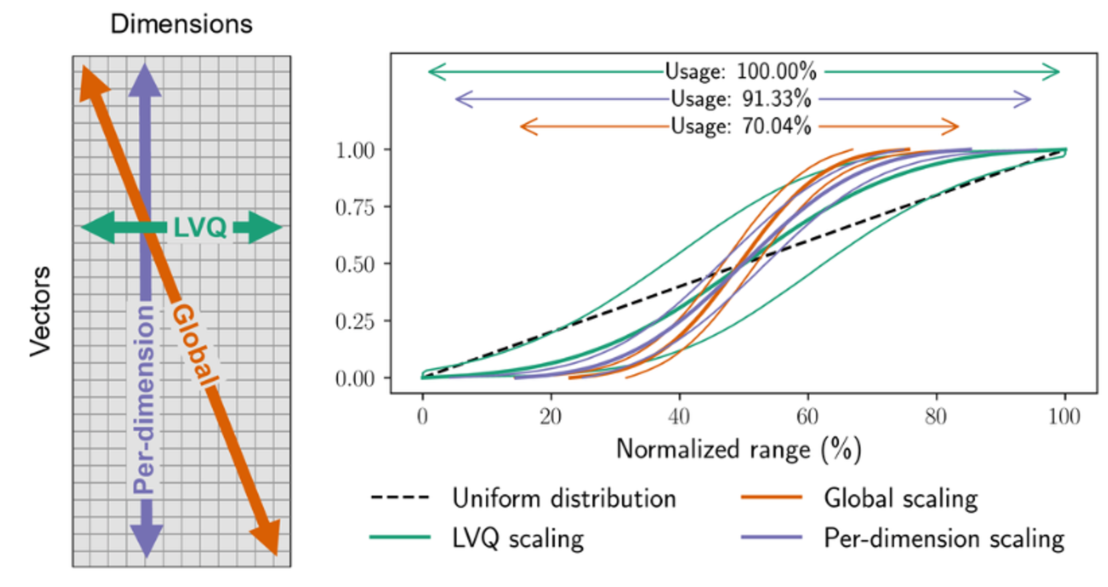
Figure 1: Empirical distributions of vector values in the deep-96-1M dataset
For 95% of the vectors, global and per-dimension normalization methods utilize only about 60% and 75% of the available value range, respectively. In contrast, LVQ normalization more closely approximates a uniform distribution, effectively using the full range and resulting in a more accurate and representative encoding. Figure from LVQ paper.
LeanVec builds on top of LVQ by first applying linear dimensionality reduction, then compressing the reduced vectors with LVQ. This two-step approach significantly cuts memory and compute costs, enabling faster similarity search and index construction with minimal accuracy loss—especially for high-dimensional deep learning embeddings.
The compression gains are substantial. LVQ achieves a four-fold reduction of the vector size while maintaining search accuracy. A typical 768-dimensional float32 vector that normally requires 3072 bytes can be reduced to just a few hundred bytes through this quantization process— this is how we can achieve 51–74% reduction in the graph index and 26-37% overall memory footprint reduction.
Two-level vector compression
For high-dimensional vectors (like the 768-dimensional embeddings common in large language models) or when maximum accuracy is required, both techniques use a two-level approach (see Figure 2). .
LVQ’s two-level compression works by first quantizing each vector individually to capture its main structure, then encoding the residual error—the difference between the original and quantized vector—using a second quantization step. This allows fast search using only the first level, with the second level used for re-ranking to boost accuracy when needed. In LVQ, LVQB₁xB₂ means the first level uses B₁ bits and the second level uses B₂ bits per vector dimension. For example, LVQ4x8 uses 4 bits for the main vector and 8 bits for the residual (i.e., a total of 12 bits per dimension).
Similarly, LeanVec uses a two-level approach: the first level reduces dimensionality and applies LVQ to speed up candidate retrieval, while the second level applies LVQ to the original high-dimensional vectors for accurate re-ranking. For example, LeanVec4x8 means the reduced-dimension vector is quantized with LVQ using 4 bits per dimension, while the original high-dimensional vector is quantized with 8 bits per dimension. Note that the original full-precision embeddings were never used by either LVQ or LeanVec, as both operate entirely on compressed representations.
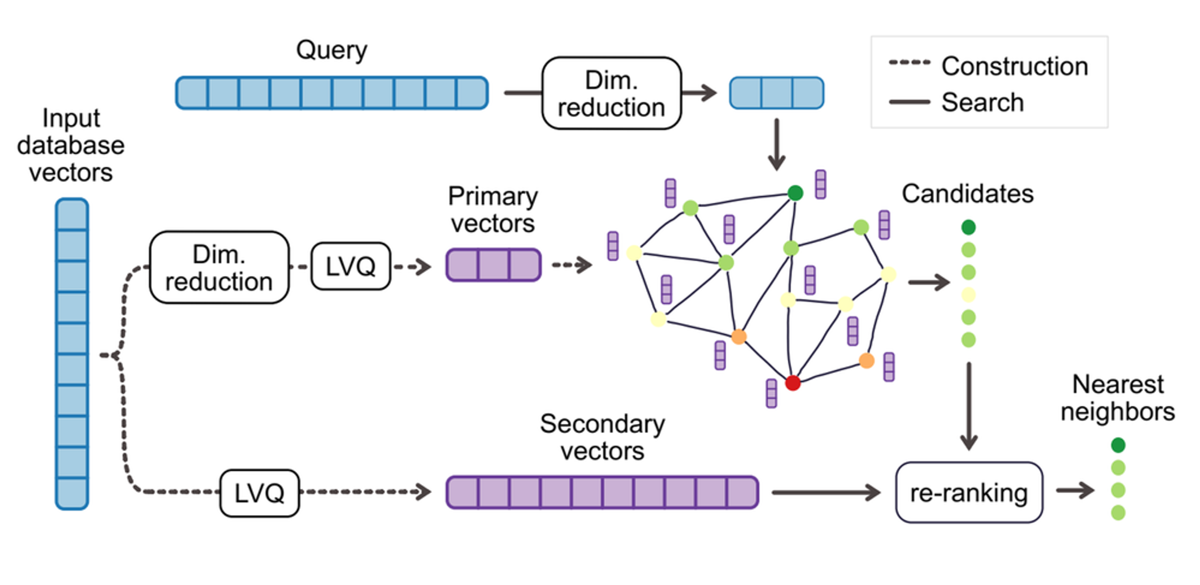
Figure 2. Two-level vector compression implementation with LVQ and LeanVec
Optimized for performance
Is this performant, since I’m doing all this computation? The engineering achievement is in the performance optimization. LeanVec improves search performance with a two-fold acceleration while operating on compressed vectors. The core performance optimization behind LVQ and LeanVec lies in their ability to maintain the sub-millisecond search times that Redis is known for while operating on a fraction of the original memory footprint. This is possible because graph-based similarity search is memory-bound—most of the time is spent fetching vectors from memory rather than computing distances. LVQ and LeanVec preserve enough accuracy that the slight increase in search effort doesn’t outweigh the gains from reduced memory bandwidth usage. As a result, the improved memory efficiency directly translates into faster search performance.
A second key factor is LVQ’s extremely low decompression overhead. Techniques like Turbo LVQ optimize the memory layout of quantized vectors to align with SIMD-friendly access patterns. Instead of storing dimensions sequentially, Turbo LVQ permutes the layout to pack 128 dimensions into 64 bytes, allowing 16 dimensions to be unpacked with just two assembly instructions—compared to seven in traditional layouts. This enables highly efficient distance computations, effectively amortizing the cost of compression during search.
Together, these optimizations allow Redis powered by SVS-VAMANA with LVQ and LeanVec to deliver fast, accurate search with a much smaller memory footprint—without ever needing to access the original full-precision vectors. Check out the rule of thumbs and what compression option suits your use case.
Leveraging Redis asynchronous vector indexing
Redis vector indexes use a tiered index architecture designed to offload the heavy computational work required for inserting and deleting elements in graph-based vector indexes such as HNSW and the new SVS-VAMANA.
In this architecture, the Redis main thread, which is responsible for handling client requests, does not perform the full insertion directly. Instead, it temporarily stores new vectors in a bounded buffer. Background worker threads then asynchronously insert those vectors into the underlying graph structure (see Figure 3).
The same principle applies to deletions: the main thread only marks vectors as deleted, while background threads handle the expensive task of repairing graph links and reclaiming memory.
A similar approach is applied when running queries, which is particularly beneficial for vector searches. By handling the heavy computation asynchronously, Redis ensures that the main thread remains responsive to other client requests. This design significantly increases both write and read throughput and enables efficient memory management, without compromising index quality or query accuracy.
Redis Query Engine integrates SVS-VAMANA using this tiered index mechanism. As a result, users can sustain heavy vector write workloads while Redis continues to remain responsive, serving queries in parallel and consistently over dynamically evolving data.
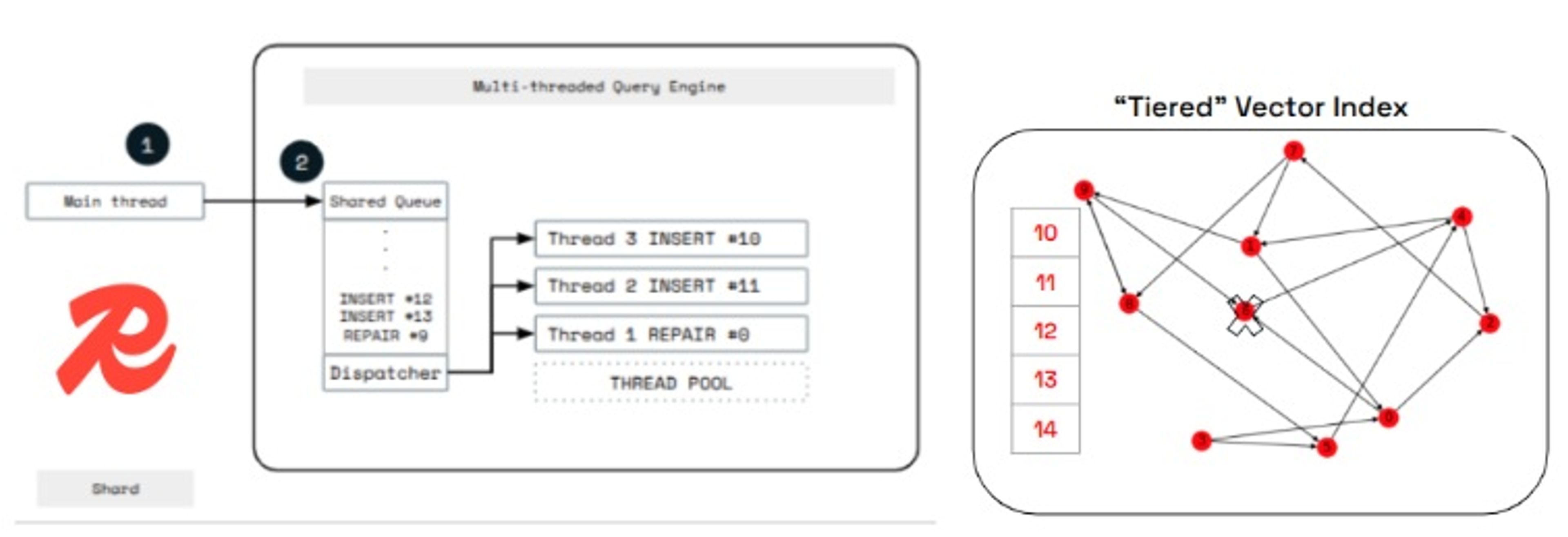
Figure 3. Redis Query Engine tiered index architecture
Benchmark comparisons for memory, throughput, latency and ingestion time
To assess SVS-VAMANA performance we’ve used the vector-db-benchmark tool, focusing on high precision and high concurrency scenarios, across 3 different datasets, and 3 different CPU vendors (Intel, AMD, and ARM) using GCP, given SVS behaves differently, i.e. uses different algorithms, depending on the underlying hardware.
- On Intel chips SVS-VAMANA can use LVQ and LeanVec, as described before. As a rule of thumb, you should use LVQ for vectors with dimensions lower than 768 and, use LeanVec for vectors with dimensions equal to or larger than 768. The benchmark methodology followed this recommendation.
- On non Intel CPUs, i.e. AMD and ARM, and on Redis Open Source version, compression will fall back to SQ8. Developers can opt-in for install the SVS optimizations on Redis Open Source follow this guide.
We’ll deep dive into memory savings, throughput, latency improvements, and ingestion tradeoffs taking into account all 3 CPU types when the data is relevant for ARM/AMD, and always compare to the HNSW baseline. Ultimately, we want you to fully understand the benefits and tradeoffs of SVS-VAMANA after reading the following section.
Memory gains
One of the most immediate benefits of the new Redis-Intel SVS compression is memory efficiency. Across all datasets we tested (detailed list on the appendix), SVS-VAMANA consistently delivered 26–37% total memory savings compared to HNSW, and when looking only at the vector index, the reductions were even more dramatic: 51–74% less memory used.
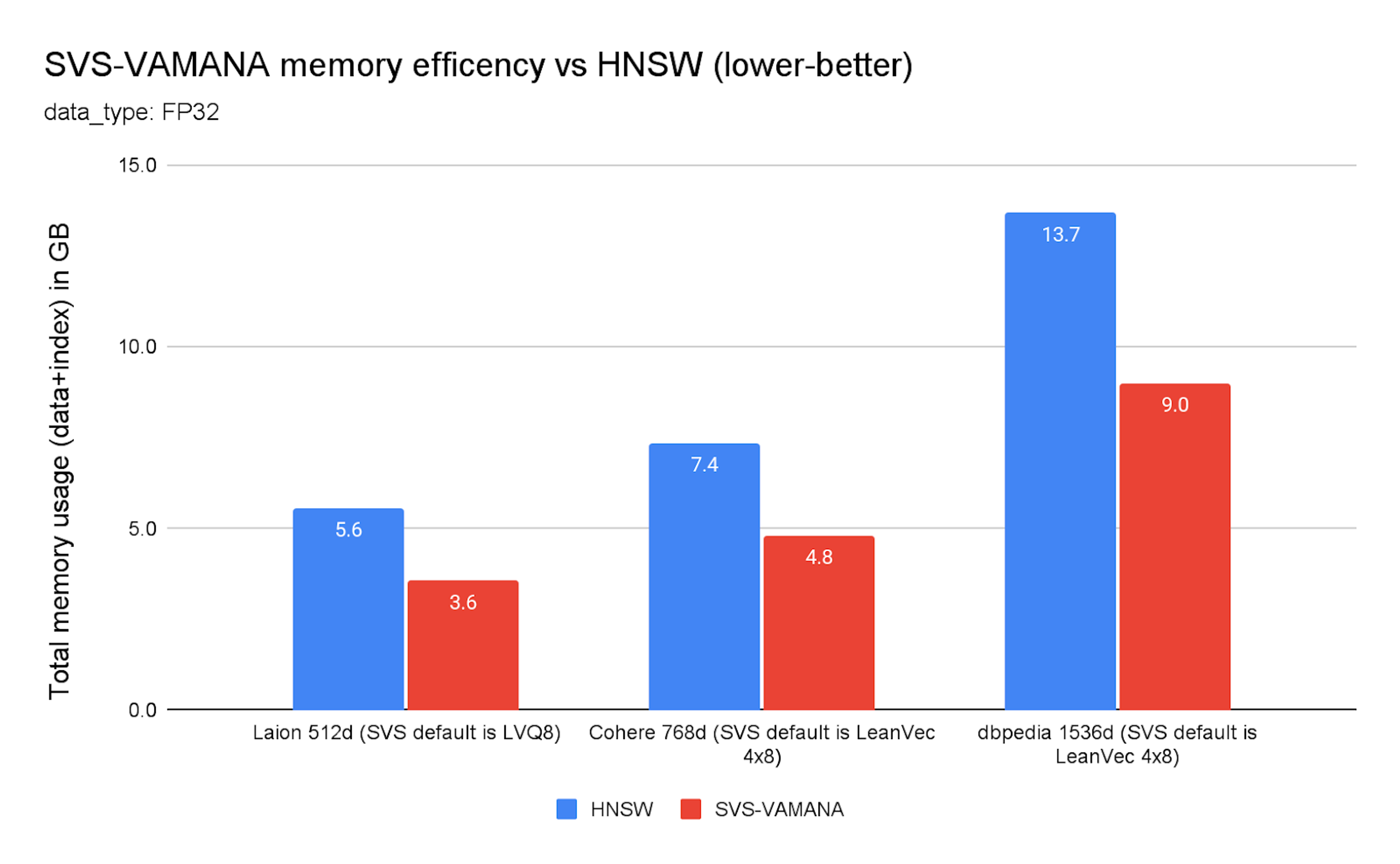
Chart 1. SVS-VAMANA memory efficiency vs. HNSW
Chart 1 highlights memory efficiency gains of SVS-VAMANA LVQ8 config per dataset compared to HNSW across multiple datasets and embedding sizes (Laion 512d, Cohere 768d, and DBpedia 1536d) for FP32 data. In every case, SVS-VAMANA significantly reduced total memory usage by up to 37%.
In practice, this means you can reduce your cloud footprint, or run larger workloads on the same hardware. SVS-VAMANA compression not only optimizes query performance, it also turns memory into a lever for cost efficiency, ensuring your vector search can scale sustainably.
Accuracy trade-off, is there any?
A natural concern with any new indexing method is whether accuracy suffers compared to HNSW. Our testing shows that it doesn’t: all SVS-VAMANA variants (LeanVec and LVQ) can match the high precision levels of HNSW, also confirming what Intel has documented in their Scalable Vector Search deep dive.
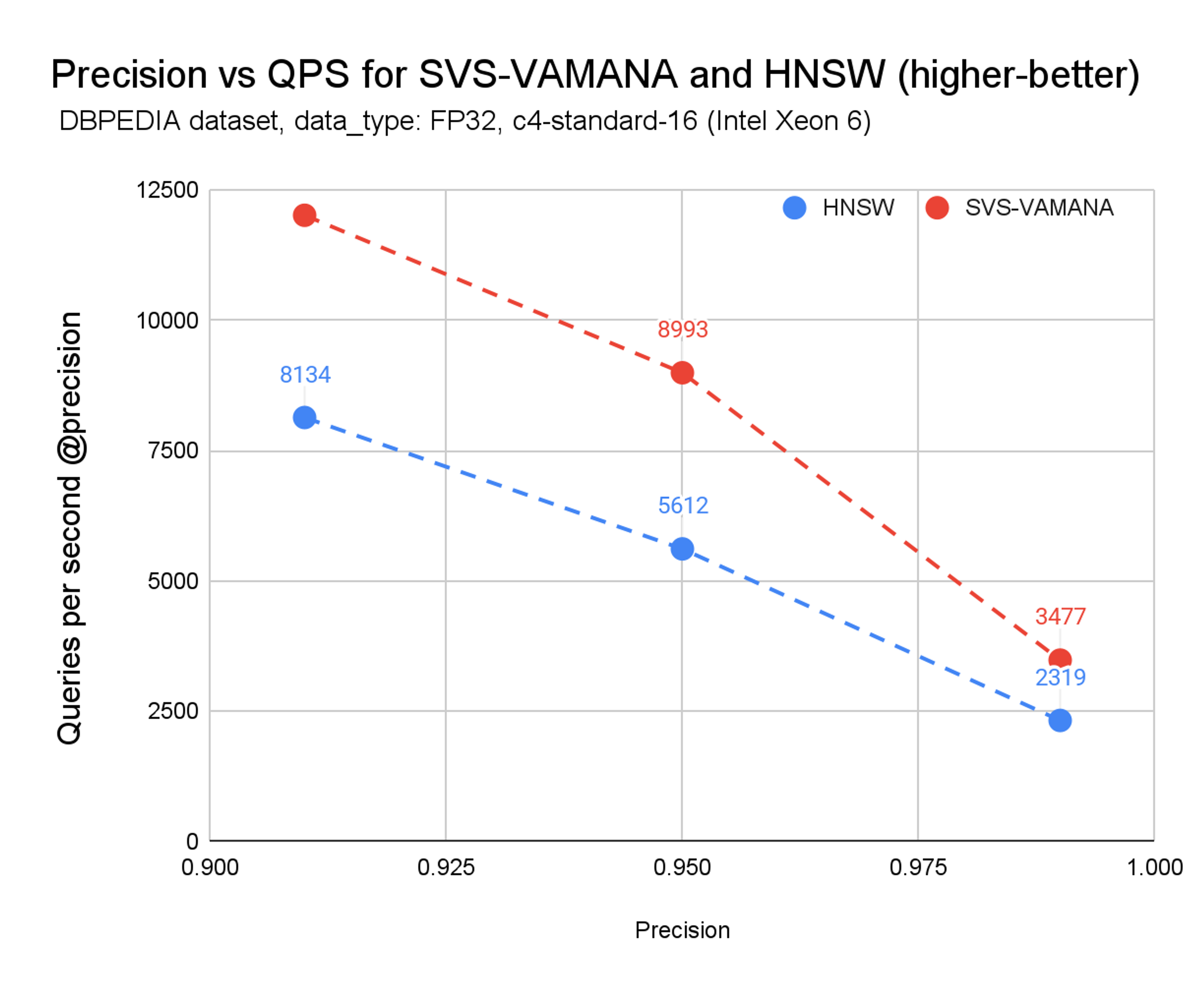
Chart 2. Precision vs. QPS for SVS-VAMANA and HNSW
From Chart 2 we can see that at t every precision point—from ~0.92 up to 0.99—SVS-VAMANA tracks alongside HNSW in accuracy while consistently delivering higher queries per second (QPS). The advantage is visible both at lower precision targets, where SVS-VAMANA pulls ahead aggressively, and at higher precision levels, where it sustains up to 1.5× better throughput at the same precision.
With SVS-VAMANA you get HNSW-grade accuracy, plus the performance and efficiency benefits on top.
Unlocking QPS and latency improvements with SVS-VAMANA
Beyond memory savings while keeping accuracy, SVS-VAMANA unlocks meaningful performance improvements in real-world search workloads. Let’s start with throughput: which cases have benefits, and which ones not that much.
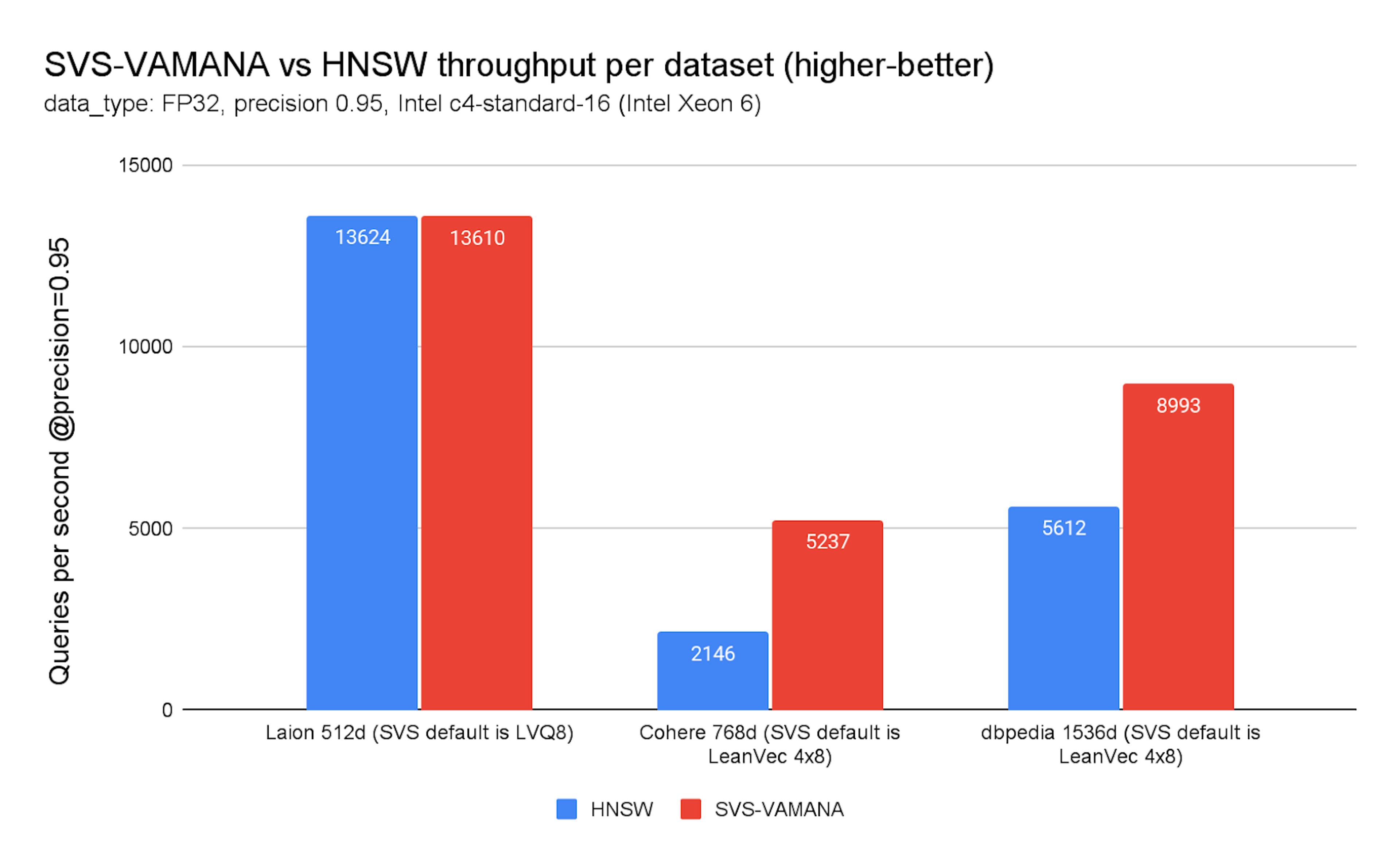
Chart 3. SVS-VAMANA vs. HNSW throughput per dataset
On FP32 datasets, throughput gains are substantial: up to 144% higher QPS on COHERE (768d, dot product) and up to 60% on DBpedia (1536d, cosine). These improvements are visible across the recommended SVS-VAMANA quantization method for vectors with dimensions equal to or higher than 768, LeanVec 4x8, and hold even at high precision thresholds (see Chart 3). You can check the COMPRESSION options and datasets details in the appendix.
Not all datasets behave the same, however. On LAION (512d, cosine), SVS-VAMANA yields only marginal improvements—0–15% in most cases, with some degradation. It’s worth noting that these results still come with a reduction in memory footprint, which can be attractive to customers even in cases without significant performance gains. This makes SVS-VAMANA most appealing for medium-to-large embedding workloads (768–3,072 dimensions), where both memory and compute savings amplify its advantages.
Throughput is only half the story. For many production workloads, what really matters is latency—how fast results come back when systems are under load. Looking at p50 and p95 latencies, SVS-VAMANA consistently outperforms HNSW, cutting response times even as query concurrency scales.
On FP32, the gains are striking: on Cohere (768d, dot product), SVS-VAMANA reduced latency by 60% at p50 and 57% at p95 compared to HNSW. DBpedia (1536d, cosine) also showed strong improvements, with 46% lower p50 and 36% lower p95, for high concurrency benchmarks (see Chart 4).
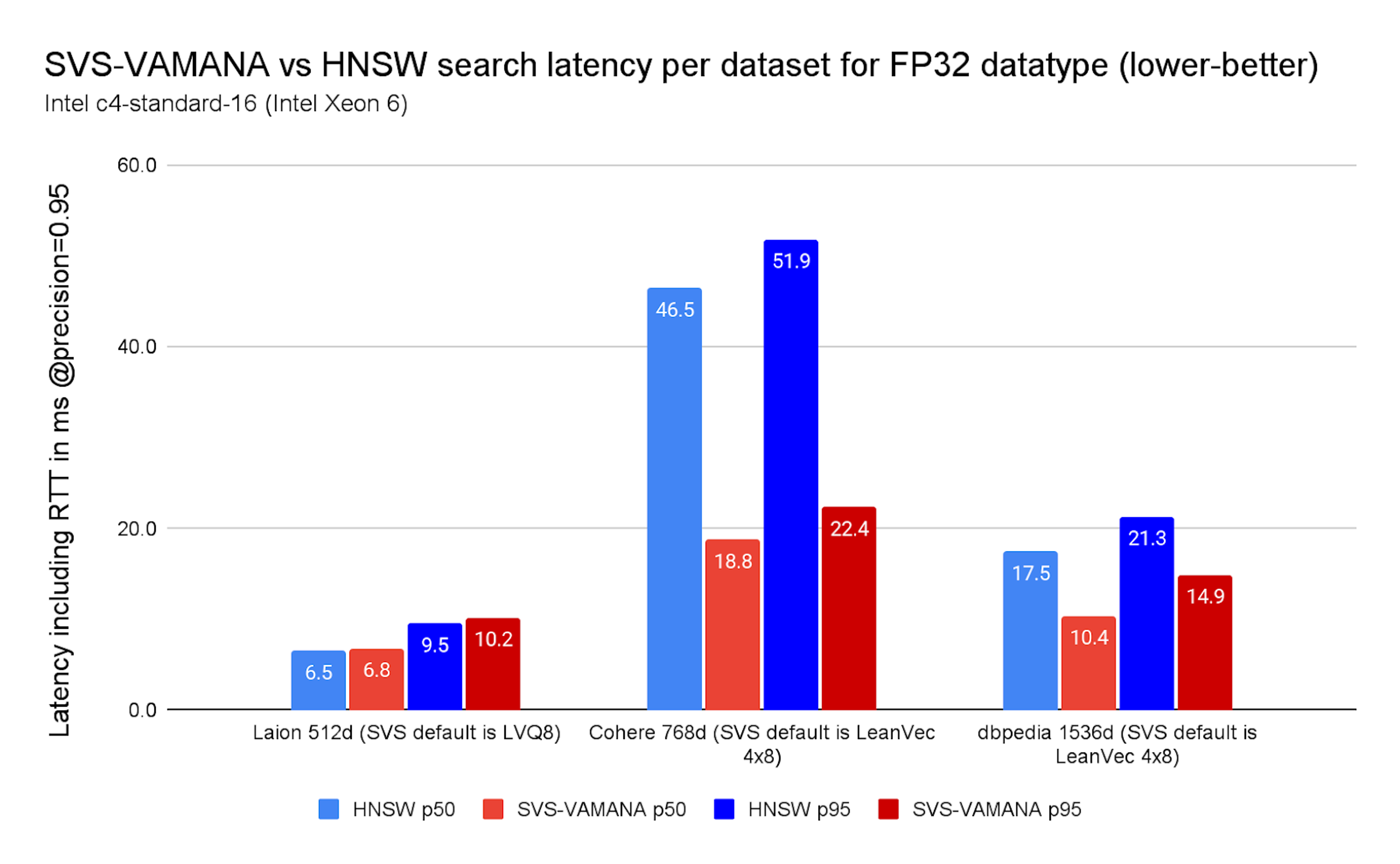
Chart 4. SVS-VAMANA vs. HNSW search latency per dataset for FP32 datatype
With FP16 (Chart 5), the picture is consistent but the drops are smaller, with the largest advantage being on Cohere dataset dropping latencies up to 43%. 43%/40% on Cohere, and 11% on DBpedia. This is expected: SVS-VAMANA accelerates search primarily by reducing memory accesses, so when each vector already consumes less memory (as with FP16) the relative advantage naturally shrinks. Even then, SVS-VAMANA still delivers meaningful latency improvements where workloads are memory-bound.
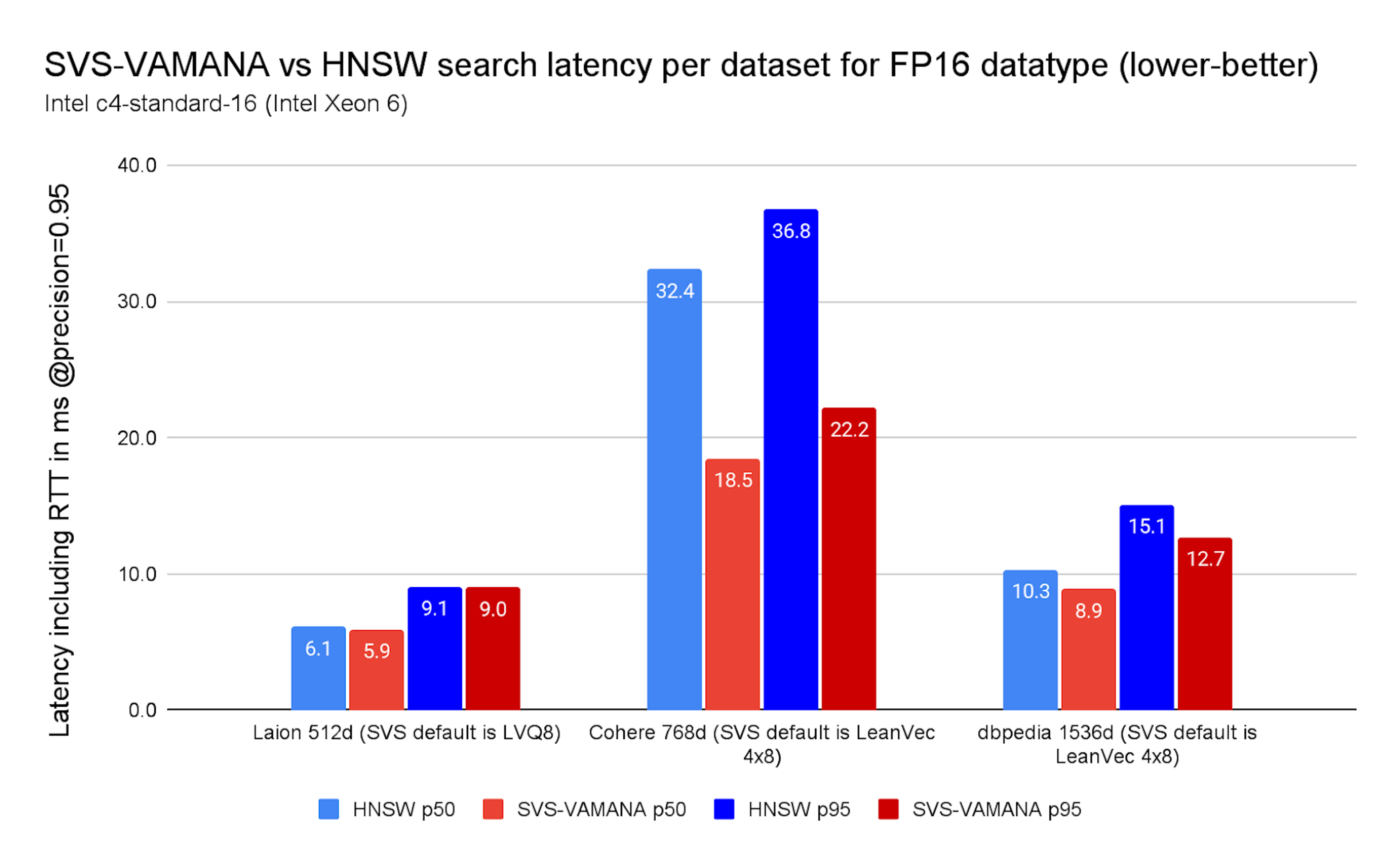
Chart 5. SVS-VAMANA vs HNSW search latency per dataset for FP16 datatype
Across datasets, these reductions translate into faster responses for end users under heavy traffic. While LAION (512d) shows little to no change on latency while still reducing memory, the medium- and high-dimensional workloads—Cohere and DBpedia—demonstrate that SVS-VAMANA not only improves throughput but also keeps response times reliably low at scale while saving memory at the same time.
For all data-dependent compression methods, the benefits naturally vary across datasets, as they are influenced by factors such as dimensionality, the structure of the embedding manifold, and overall compressibility. Cohere and DBpedia, being higher-dimensional, show greater benefits than LAION. Differences between Cohere and DBpedia likely stem from variations in their embedding manifolds. Even though LAION shows smaller gains, it still maintains performance while using significantly fewer bits—half compared to float16 and a quarter compared to float32—demonstrating the strength of LVQ compression.
Ingestion trade-offs – computing compression
The main cost of SVS-VAMANA lies in ingestion. To illustrate it, we’ve selected 2 datasets, one for each SVS-VAMANA variant (LAION for SVS LVQ8 and DBPEDIA for LeanVec 4x8), see Chart 6 and Chart 7.
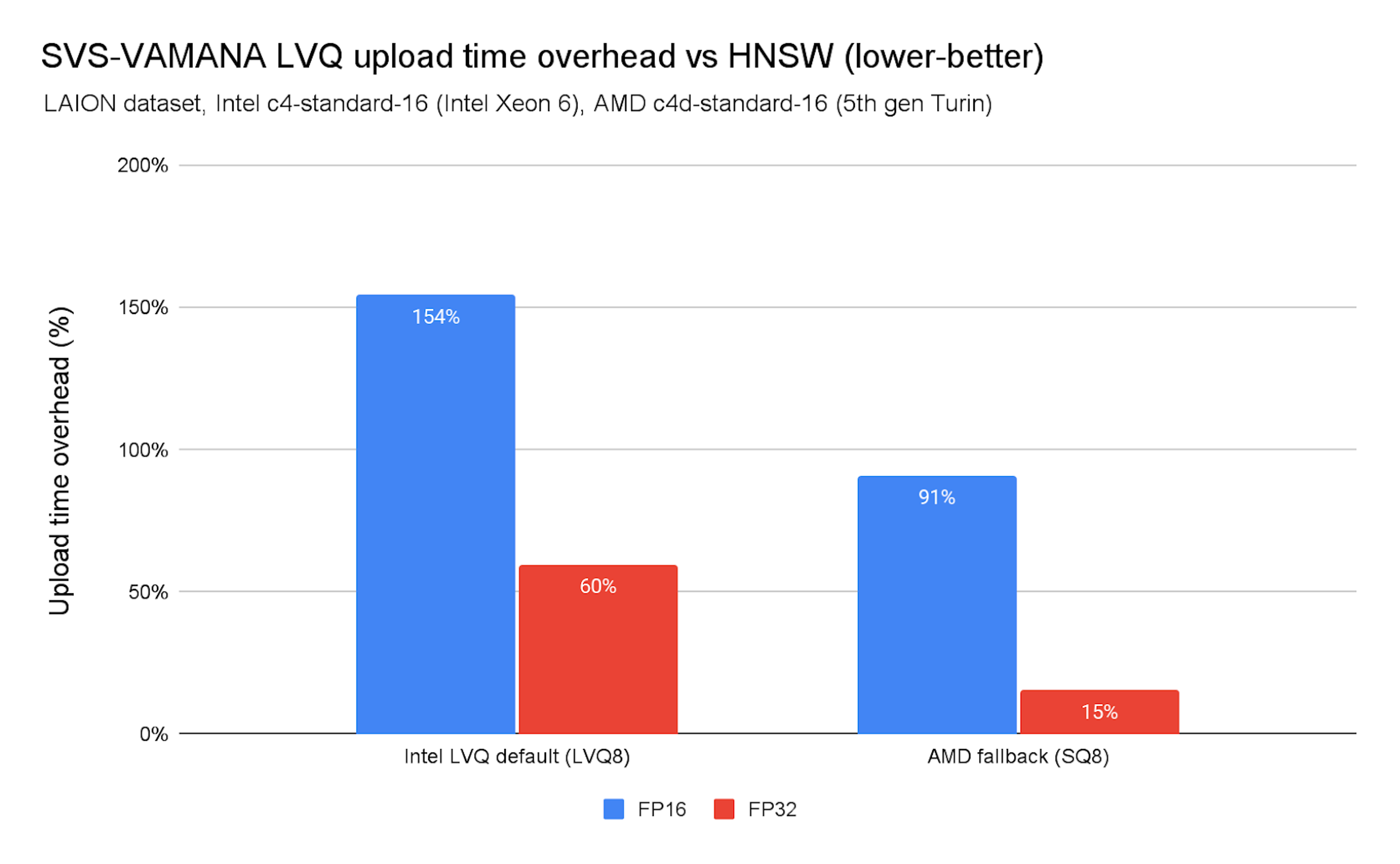
Chart 6. SVS-VAMANA LVQ upload time overhead vs. HNSW
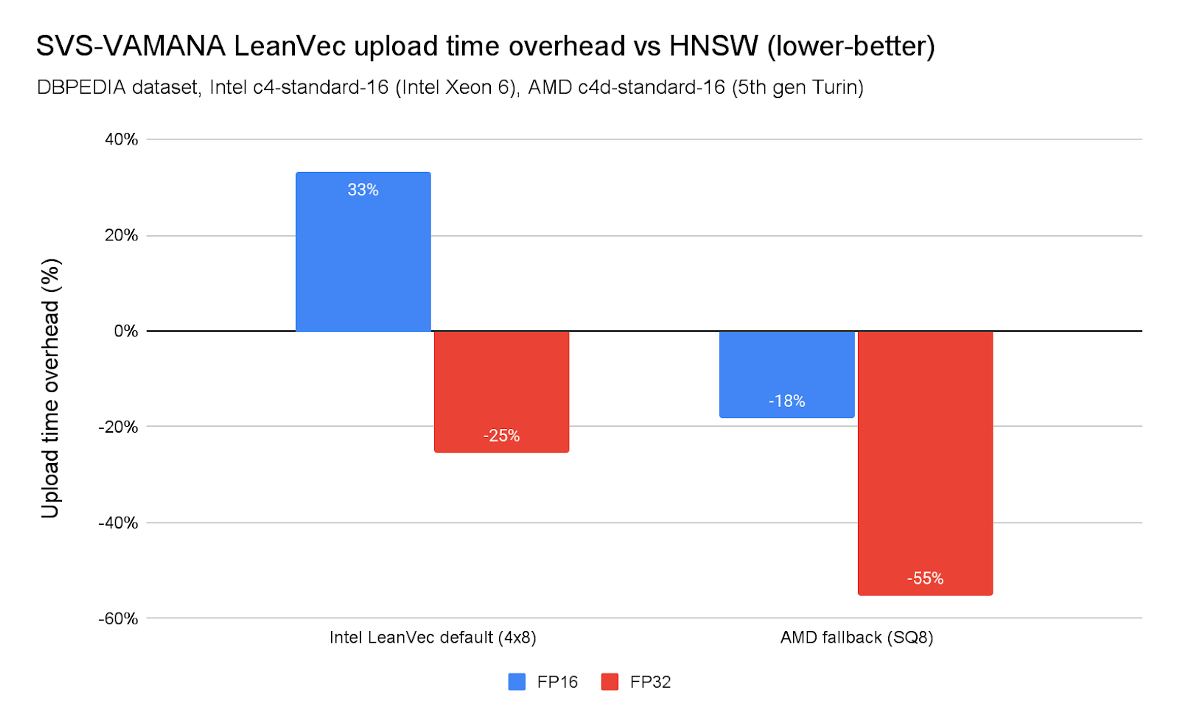
Chart 7. SVS-VAMANA LeanVec upload time overhead vs. HNSW
As shown in Chart 7, index construction times are higher than HNSW. On x86 platforms (Intel and AMD) the overhead is manageable.
SVS-VAMANA is currently not optimized for ingestion performance, so slowdowns compared to HNSW are expected. These differences stem from several factors, including the additional overhead introduced by vector compression, differences in the graph edge pruning strategies used in each algorithm, and the concurrency control approach used in SVS-VAMANA, which relies on a global lock during ingestion.
Ingestion with LeanVec is generally faster than with LVQ, primarily because search is significantly faster with LeanVec, which typically operates on dimensionally reduced vectors quantized with 4 bits per dimension—resulting in highly compressed representations. We plan to investigate these aspects further and work on targeted optimizations for future releases.
For Intel:
- LeanVec can accelerate upload times in some cases (e.g., up to 25% faster on Intel FP32), but it may also be up to 33% slower depending on the dataset. These differences stem mostly from how dataset characteristics like dimensionality, embedding structure, and compressibility influence the effectiveness of data-dependent compression methods.
- LVQ is generally slower, with ingestion times reaching up to 2.6× longer than HNSW.
For AMD, the fallback algorithm (SQ8) showcased either improvements on the upload time for FP32 or small regressions depending on the configuration. Nonetheless, and as mentioned above, the overhead is smaller.
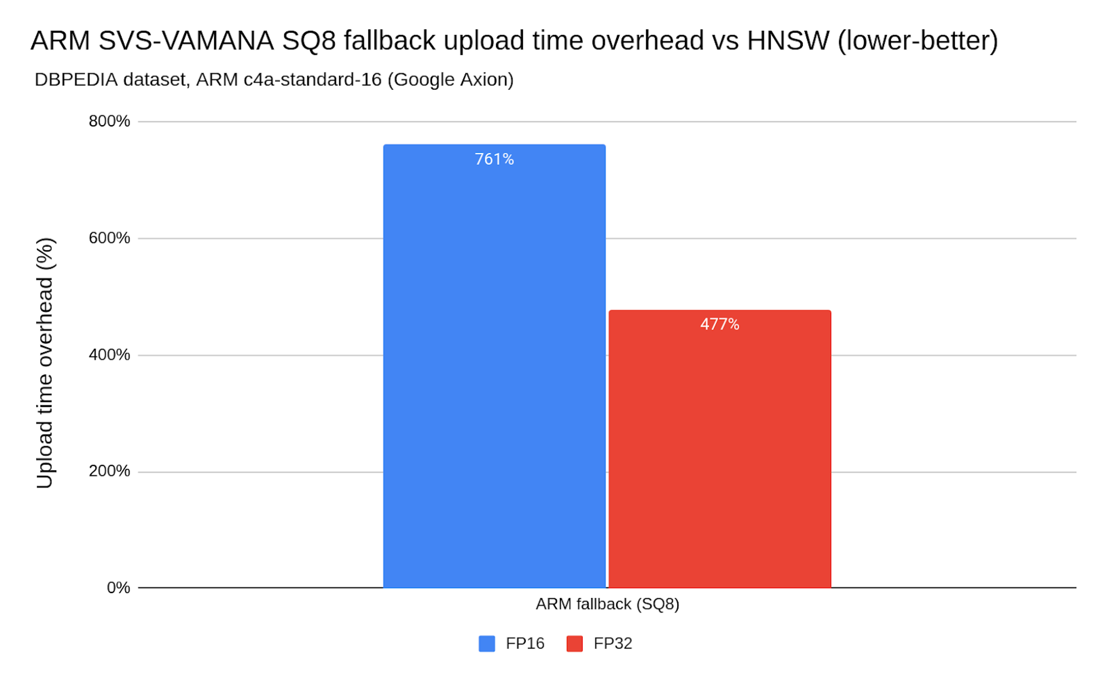
Chart 8. ARM SVS-VAMANA SQ8 fallback upload time overhead vs. HNSW
On ARM, the story is different. Ingestion times can be 9× slower (see Chart 8) than HNSW, making SVS-VAMANA impractical on ARM platforms today. This gap is less about ARM hardware capabilities and more about the fact that SVS-VAMANA optimizations are primarily tuned for x86, and the fallback algorithm (SQ8) is not optimized for ARM. In other words, SVS-VAMANA and its fallback, isn’t yet optimized for ARM ingestion workloads.
Comparison with other CPUs. Choosing the right fit
Our benchmarks show that the best algorithm depends on the underlying hardware, considering the regular quantization (SQ8 fallback) versus Intel optimizations. Both x86 (Intel and AMD) and ARM have strengths — but they shine in different ways.
To prove it, we’ve charted below (Charts 9 and 10) the achievable QPS at a 0.95 precision for the DBPEDIA dataset across Intel (c4), AMD (c4d), and ARM (c4a) instances on GCP. We also included an additional SVS-VAMANA configuration tuned for performance, LeanVec Dimensions/4, obtained by setting REDUCE, the target dimension used in the dimensionality reduction step, to 384 (i.e., dim/4 = 1536/4 = 384).
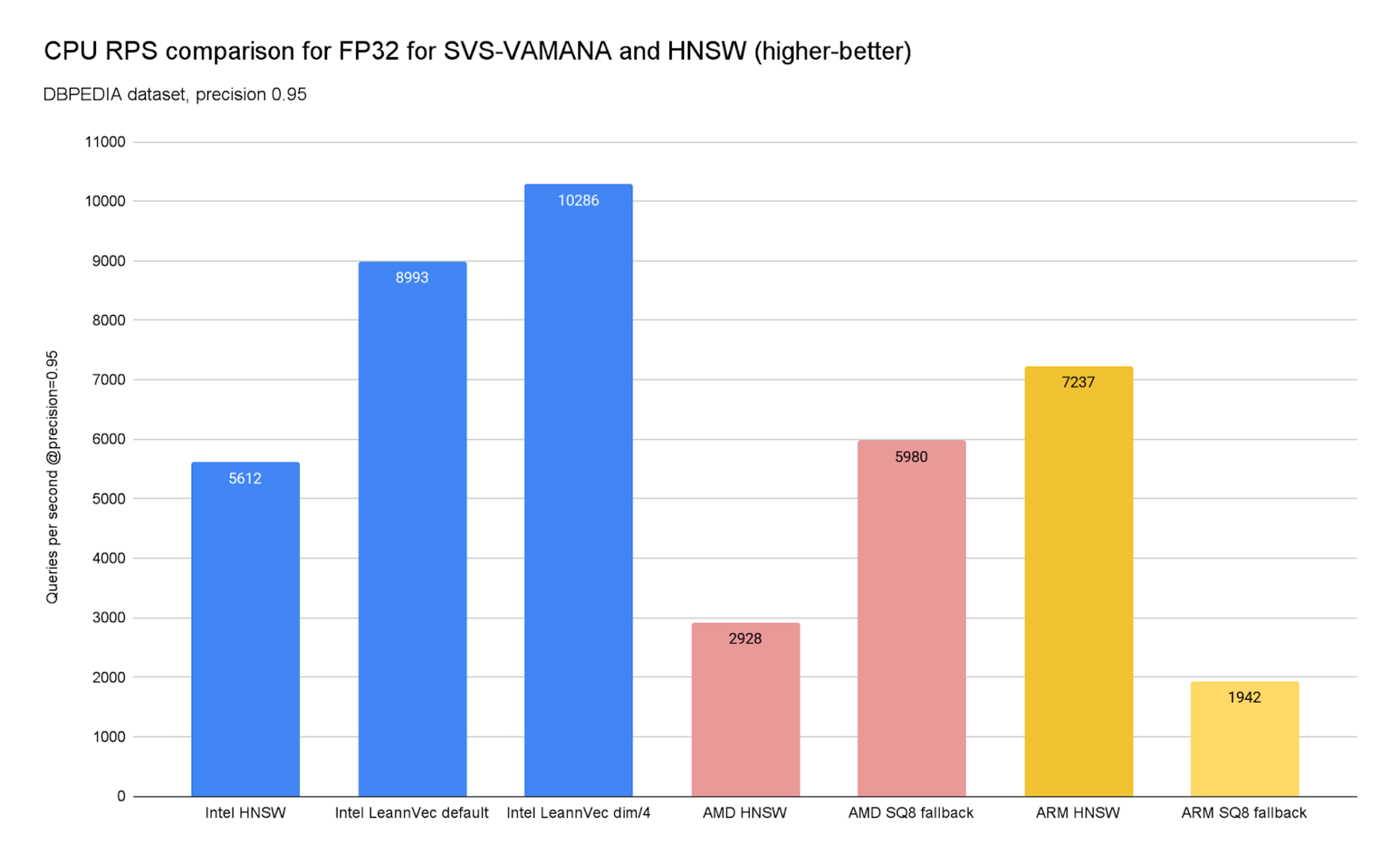
Chart 9. CPU RPS comparison for FP32 for SVS-VAMANA and HNSW
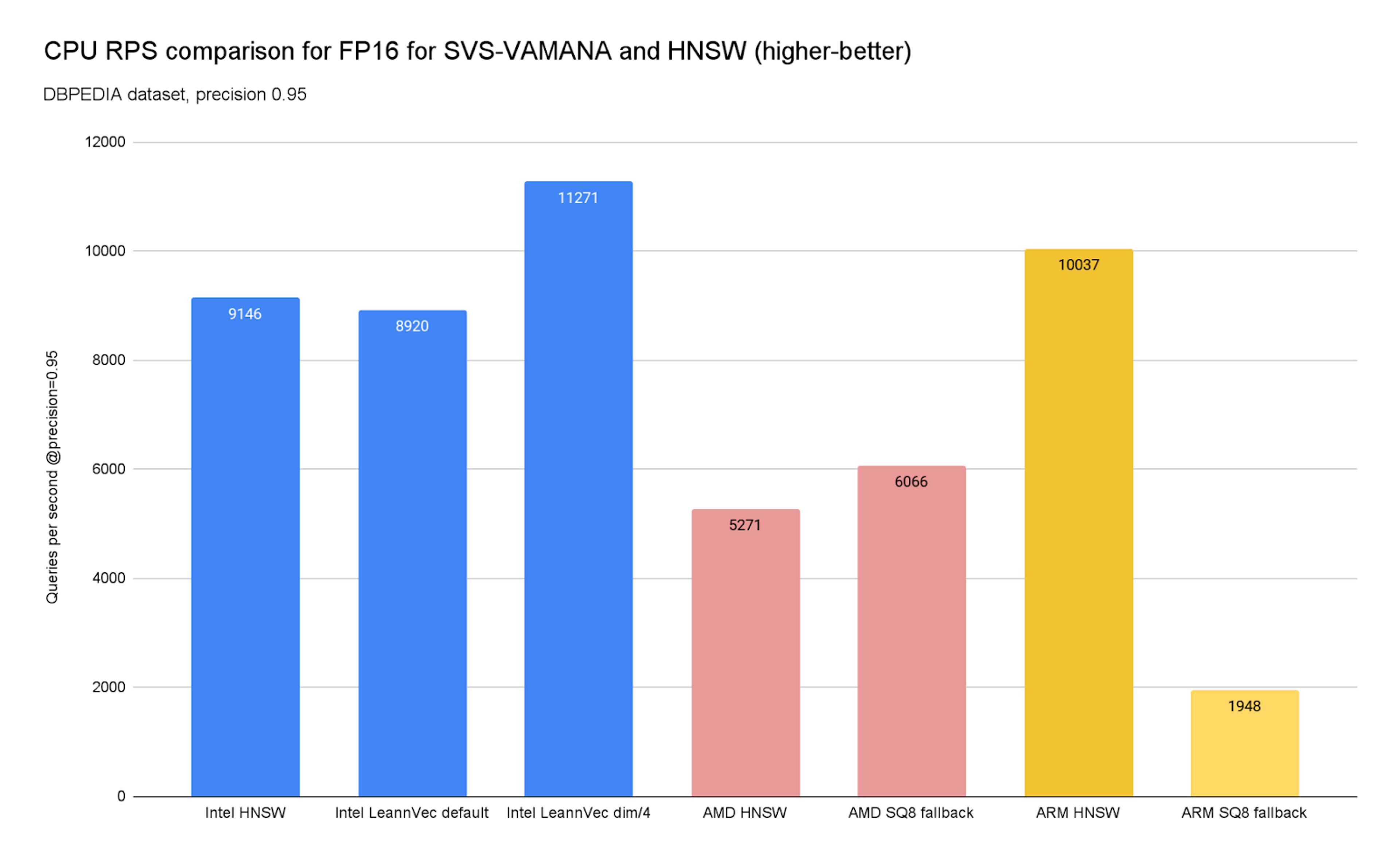
Chart 10. CPU RPS comparison for FP16 for SVS-VAMANA and HNSW
The results confirm a clear theme: the best algorithm depends heavily on the underlying hardware.
On x86 platforms, SVS-VAMANA really comes into its own. On Intel platforms, large performance gains are achieved by leveraging Intel's compression technologies, while on AMD, strong performance is enabled through the SQ8 fallback, delivering:
- Higher query throughput — up to 144% improvement over HNSW in some datasets.
- Lower latency — p50 and p95 reduced by up to 60%.
- Smaller memory footprint — 26–37% less overall memory, 51–74% less index memory.
For high-throughput, FP32 workloads where performance and memory efficiency matter most, x86 + SVS-VAMANA is the recommended configuration.
Furthermore, the performance-tuned LeanVec dim/4 configuration improves ingestion time, always outperforming HNSW.
On ARM platforms, the story is different. ARM already runs HNSW exceptionally well — in fact, our benchmarks show ARM HNSW can even edge ahead of x86 HNSW by ~10% in search throughput depending on the use-case. For teams standardizing on ARM infrastructure, this means you can achieve competitive performance with HNSW at lower cost and power efficiency, and that the fallback algorithm on ARM, which is Scalar Quantization 8, is not yielding better results than HNSW.
Today, SVS-VAMANA on ARM does not yet match its x86 performance. Upload times are longer, and query throughput lags behind Intel and AMD. This is primarily due to the lack of ARM-native vector acceleration for SVS-VAMANA and an optimized implementation of the fallback algorithm used (SQ8 like mentioned previously). However, ARM’s excellent HNSW results make it a strong choice for production workloads until further optimizations arrive.
Takeaway:
- If you are on x86, SVS-VAMANA offers top-tier speed, latency, and memory savings—delivering major gains on Intel and strong results on AMD even without the optimized version.
- If you’re on ARM, HNSW continues to be the go-to option — delivering competitive search performance and excellent efficiency.
Differences in configurations and comparison of benefits for LVQ & LeanVec
From a developer perspective, new Redis SVS-VAMANA integrates seamlessly into your existing Redis workflows. When creating vector indices with FT.CREATE, you can now specify the new SVS-VAMANA algorithm along with compression options directly in your VECTOR field definitions.
As mentioned in the previous sessions, the ultimate gains came from Intel hardware optimizations (LVQ and LeanVec), while in others platforms the option always falls in a regular quantization method using 8-bit (SQ8). For developers, it’s transparent, since the optimization is triggered in Redis Enterprise as soon as the Intel hardware is detected.
Code on Redis Open Source, using regular SQ8 and leverage the optimizations for Intel on Enterprise. Please check the documentation instructions on how to trigger the optimizations also on Redis Open Source.
Note:
Here's how simple it is to enable COMPRESSION using SVS-VAMANA:
```
FT.CREATE myindex SCHEMA
embedding VECTOR SVS-VAMANA 6
COMPRESSION LVQ8
TYPE FLOAT32
DIM 768
DISTANCE_METRIC COSINE
```
On the query side, your application code remains unchanged—the same search commands return the same high-quality results, just with improved memory efficiency. The quantization happens transparently during indexing, and Redis Query Engine handles all the complexity of encoding, storage, and fast similarity computation.
Whether you're working with FLOAT16 or FLOAT32 vectors, compression is supported across both data types, giving you the flexibility to choose the precision that best fits your application requirements while still benefiting from the memory savings.
In order to understand better what compression to use, it’s important to understand the different embedding options and applications for a given use case see Figure 4.
Common embedding types & their characteristics
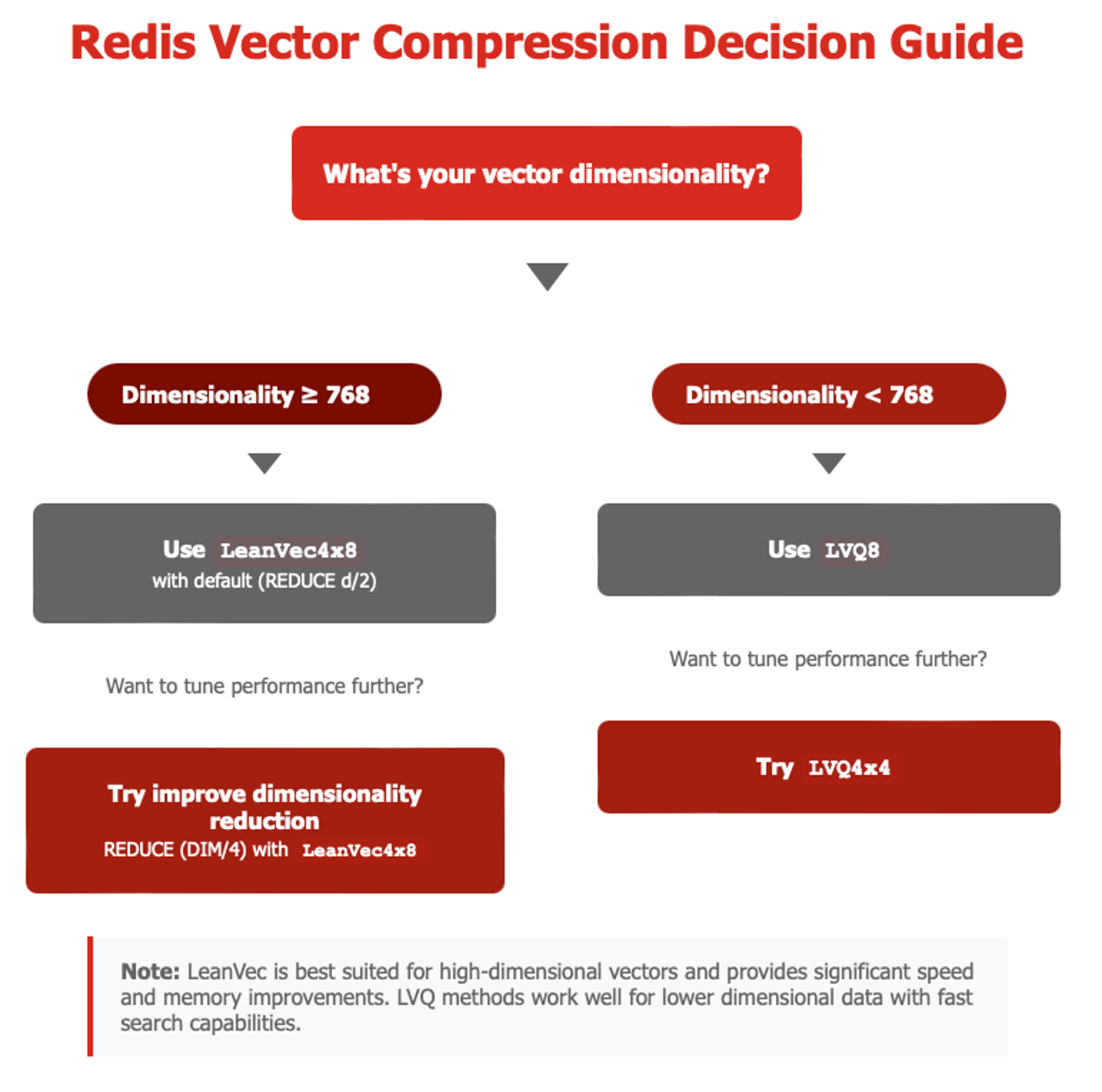
Figure 4. Decision tree for selecting the right quantization
Different embedding models create vectors with distinct properties that affect quantization and compression performance:
- Text Embeddings (OpenAI, BERT, Cohere, SentenceTransformers): These models typically produce 384 to 1536-dimensional vectors that are dense and semantically rich.
- Image Embeddings (CLIP, ResNet, ViT): Usually exceeding 1024 dimensions, these vectors exhibit higher variability and noise due to the complexity of visual data.
- Multimodal Embeddings (CLIP, unified models): These vectors combine text and image characteristics, creating mixed data patterns that often require more sophisticated quantization strategies to preserve recall across different modalities.
- Custom Embeddings (anomaly detection, feature engineering): Domain-specific vectors may need calibration or profiling to determine optimal quantization settings, but SVS-VAMANA adaptive approach typically handles these variations effectively.
The SVS-VAMANA with LVQ and LeanVec configurations reflects the number of bits allocated per dimension at each level of compression.
Naming convention: LVQ<B₁>x<B₂>
B₁: Number of bits per dimension used in the first-level quantization.
B₂: Number of bits per dimension used in the second-level quantization (residual encoding).
| LeanVec | Combines dimensionality reduction with LVQ, applying quantization after reducing vector dimensions. | LeanVec4x8, LeanVec8x8 |
As an example, we elaborate in Table 1 with different embedding types and use cases, and the suggested Compression to use. Depending on the type and dimensionality chosen, these numbers may vary considerably.
| Text Embeddings | Document search, semantic similarity, Q&A systems | Cohere embed-multilingual-v3 (1024) OpenAI text-embedding-ada-002 (1536) | LeanVec 4x8 (following REDUCE adjustments if required) | ~3x compression |
| Image Embeddings | Visual similarity search, content-based retrieval | ResNet-152 (2048) | LeanVec 4x8 | ~3x compression |
| Multimodal | Cross-modal search, unified content systems | CLIP ViT-B/32 (512) | LVQ8 | ~3.5x compression |
| Custom/Domain | Anomaly detection, specialized feature matching | Cohere embed-v3 (1024) | LeanVec 4x8 | ~3x |
Table 1. Compression strategy per use-case.
While optimizing the memory footprint using vector compression, it may require slightly changing the `SEARCH_WINDOW_SIZE` (equivalent to HNSW’s `EF_RUNTIME`) to match search accuracy. See the entire list of advanced parameters for tuning the Index and Query in our documentation.
Building the future
On our road to sustain our tripod of speed, accuracy and cost, we will keep extending the coverage of a comprehensive compression, leveraging multiple techniques for other indexes, such as HNSW, and index types. As part of our partnership with Intel, we plan to incorporate other SVS library optimizations into the Redis Query Engine. One key enhancement is the use of LeanVec for handling out-of-distribution (OOD) queries—a major challenge in cross-modal retrieval—through a query-aware dimensionality reduction approach.
Multi-vectors support is also part of the roadmap, which brings different challenges in keeping memory footprint and computing efficiency.
Key takeaways
- Product quantization and scalar quantisation with global constants alone don't do the magic
- If you’re on x86, SVS-VAMANA unlocks the best combination of speed, latency, and memory savings.
- If you’re on ARM, HNSW continues to be the go-to option — delivering competitive search performance and excellent efficiency.
- Rule of Thumb: Leverage LeanVec for high-dimensional vectors (>=768) while LVQ will be better suitable for smaller dimensionality vectors (<768)
Acknowledgments
We would like to acknowledge the outstanding collaboration between Intel and Redis in bringing the Intel SVS library into the Redis Query Engine. From Intel, Aaron Lin, Ishwar Bhati, Mihai Capotă, Cecilia Aguerrebere, Ethan Glaser, Andreas Huber, Yue Jiao, Nikolay Petrov, Alexander Andreev, Maria Petrova, Sergey Yakovlev, Martin Dimitrov, Marcin Pozniak, Rafik Saliev, and Maria Markova contributed their deep expertise in optimization, quantization, and systems engineering. From Redis, Alon Reshef, Meirav Grimberg, Dor Forer, Omer Lerman, Adriano Amaral, Manvinder Singh, Pieter Caillaiu, Filipe Oliveira, Paulo Souza, Nathan Dunford, and Patrick Campbell worked closely to integrate and validate these capabilities. This joint effort has resulted in significant memory savings and performance improvements, advancing the state of vector search within Redis.
Appendix: Datasets and compression used
We used datasets representing various use cases.
We selected the following datasets to cover a wide range of dimensionalities and distance functions. This approach ensures that we can deliver valuable insights for various use cases, from simple image retrieval to sophisticated text embeddings in large-scale AI applications.
| laion-img-emb-512-1M-cosine | 1,000,000 | 512 | Cosine | Image embeddings derived from the LAION-5B dataset. |
| cohere-768-1M | 1,000,000 | 768 | Dot Product | English Wikipedia embeddings generated with Cohere’s multilingual encoder. |
| dbpedia-openai-1M-angular | 1,000,000 | 1536 | Cosine | OpenAI’s text embeddings dataset of DBpedia entities, using the text-embedding-ada-002 model. |
Table 2. Datasets
Compression configurations
Below you can find the index build and runtime configuration parameters used in our benchmarks, covering the different compression strategies evaluated.
During the query stage of the benchmarks , EF_RUNTIME (for HNSW) and SEARCH_WINDOW_SIZE (for SVS-VAMANA) are automatically tuned during calibration until the search reaches 0.95 precision.
| HNSW | None | M = varied from 16 to 32; EF_CONSTRUCTION = 200 | EF_RUNTIME varied to reach @0.95 precision in the benchmark tool. |
| SVS-VAMANA LVQ8 | LVQ8 | GRAPH_MAX_DEGREE = varied from 32 to 64; CONSTRUCTION_WINDOW_SIZE = 200 | SEARCH_WINDOW_SIZE calibrated to reach @0.95 precision in the benchmark tool. |
| SVS-VAMANA LVQ4x8 | LVQ4x8 | GRAPH_MAX_DEGREE = varied from 32 to 64, CONSTRUCTION_WINDOW_SIZE = 200 | SEARCH_WINDOW_SIZE calibrated to reach @0.95 precision in the benchmark tool. |
| SVS-VAMANA LVQ4x4 | LVQ4x4 | GRAPH_MAX_DEGREE = varied from 32 to 64; CONSTRUCTION_WINDOW_SIZE = 200 | SEARCH_WINDOW_SIZE calibrated to reach @0.95 precision in the benchmark tool. |
| SVS-VAMANA LeanVec4x8 | LeanVec4x8 | GRAPH_MAX_DEGREE = varied from 32 to 64; CONSTRUCTION_WINDOW_SIZE = 200 | SEARCH_WINDOW_SIZE calibrated to reach @0.95 precision in the benchmark tool. |
| SVS-VAMANA LeanVec4x8-div/4 | LeanVec4x8 (REDUCE = dim/4) | GRAPH_MAX_DEGREE = varied from 32 to 64; CONSTRUCTION_WINDOW_SIZE = 200 | SEARCH_WINDOW_SIZE calibrated to reach @0.95 precision in the benchmark tool. |
Table 3. Benchmarking configuration parameters.


